by Ben Edelman

This is the first installment of a three-part series of posts on quantum Hamiltonian complexity based on lectures given by the authors in Boaz and Tselil’s seminar. The second installment is here, and the third installment is here.

Quantum Hamiltonian complexity is a growing area of study that has important ramifications for both physics and computation. Our hope is that these three posts will provide an accessible (and incomplete) preview of the subject for readers who know the basics of theoretical computer science and quantum information. Much of the material is adapted from an excellent survey by Gharibian et al..

In a nutshell, quantum Hamiltonian complexity is the study of the local Hamiltonian problem. Why is this problem important enough to justify the existence of an entire subfield? To illustrate why, here are two informal characterizations of it:

To a physicist, the local Hamiltonian problem is a formalization of the difficulty of simulating and understanding many-particle quantum systems. There are deep connections between the complexity of this problem and the amount of quantum entanglement in a system. In practical terms, physicists would love to be able to solve this problem on a regular basis, and they’ve developed a rich theory of heuristics to that end.
To a computer scientist, the local Hamiltonian problem is the quantum version of constraint satisfaction problems. Any CSP can be written as a local Hamiltonian problem; and just as constraint satisfaction is the prototypical NP-complete problem by the Cook-Levin theorem, the local Hamiltonian problem plays the equivalent role for QMA (a quantum analogue of NP) by the “quantum Cook-Levin theorem.” The connections to classical complexity go on… there is even a quantum PCP conjecture!

But let’s take a step back and start at the beginning. To make sure we understand what a quantum Hamiltonian is and why it is important, it will be instructive to briefly rehash some of the fundamentals of classical statistical mechanics.

Classical energy and ground states

In the classical world, a physical system can be in any one of various states $x \in \mathcal{X}$ , each of which is a vector, with different coordinates representing different particles. Every state of the system has an energy, given by an energy function $E: \mathcal{X} \to \mathbb{R}$ . For example, in the classic Ising model of ferromagnetism, $\mathcal{X} = \{\pm 1\}^n$ . Each coordinate $x_i$ represents the spin of atom $i$ , and atoms $i$ and $j$ interact with each other whenever $(i,j)$ is an edge in a graph $G$ , which is usually a low-dimensional lattice. Energy for this system is defined as $E(x) = \sum_{(i,j) \in G}-x_i x_j$ .

Suppose we ignore our system for a long time, letting it interact with its external environment until, in the limit, it reaches thermal equilibrium at temperature $T$ . Then the probability the system is in state $x$ is given by Boltzmann’s distribution: $\Pr[x] = \frac{e^{-\beta E(x)}}{Z}$ , where $\beta \propto 1/T$ and $Z$ is the partition function required to normalize the probabilities. As the temperature tends to infinity, this distribution will approach the uniform distribution over $\mathcal{X}$ , and as the temperature tends to absolute zero, the distribution will approach the uniform distribution over the states with minimum energy. We call these minimum energy states ground states, and we call their energy the ground state energy. If we want to calculate something about a system, then it is often crucial to know the ground states and ground state energy of the system. Going back to our example, the Ising model has two ground states whenever $G$ is connected. These are the states $(+1,+1,\ldots,+1)$ and $(-1,-1,\ldots,-1)$ in which all atoms have the same spin. The ground state energy is $-|\{i,j:(i,j) \in G\}|$ .

Quantum Hamiltonians

A quantum Hamiltonian is essentially the quantum analogue of the classical energy function. Unlike with classical systems, when a quantum system is in a given $n$ -qubit state $\left|\psi\right\rangle$ , it doesn’t have a determinate energy. Instead, when we measure the energy, the value we obtain may be probabilistic and will correspond to one of the eigenvalues of the observable matrix for energy. This Hermitian matrix, denoted $H \in (\mathbb{C}^2)^{\otimes n} \times (\mathbb{C}^2)^{\otimes n}$ , is the quantum Hamiltonian, and just as the energy function characterizes a classical system, the Hamiltonian characterizes a quantum system. For a given eigenvector $|\lambda_i\rangle$ of $H$ with eigenvalue $\lambda_i$ , when we measure the energy of $|\psi\rangle$ we obtain the result $\lambda_i$ with probability $\langle\psi|\lambda_i\rangle$ , and the system collapses to the state $|\lambda_i\rangle$ (assuming the eigenvalue $\lambda_i$ has multiplicity 1). Thus, the ground state and ground state energy of a quantum system with eigenvalue $H$ are the minimum eigenvalue $\lambda_0$ of $H$ and the corresponding eigenvector $|\lambda_0\rangle$ .

The Boltzmann distribution also has a quantum analogue. A quantum system at thermal equilibrium will be in the following mixed state: $\rho_{\text{eq}} = \frac{e^{-\beta H}}{Z}$ . As the temperature approaches absolute zero, $\rho_{\text{eq}}$ will approach a superposition over the ground states.

Not only does the Hamiltonian tell us the energy of a system, it also describes the time evolution of the system (as long as it is closed). Schrödinger’s equation states that $-i \hbar \frac{d|\psi\rangle}{dt} = H|\psi\rangle$ , where $\hbar$ is Planck’s constant and $t$ is time. Thus, if a closed system is in the state $|\psi\rangle_0$ at time 0, its state at time $t$ will be $|\psi\rangle_t = e^{-itH/\hbar}|\psi\rangle_0$ . Since $H$ is Hermitian, $e^{-itH/\hbar}$ is unitary, which is another way of saying that quantum mechanical states are subject to unitary evolution.

The Local Hamiltonian problem

As we have seen, understanding the Hamiltonian of a quantum system is crucial for understanding both the system’s equilibrium behavior and its time evolution. There are a huge variety of questions physicists are interested in asking about systems, all of which boil down to questions about equilibrium behavior, time evolution, or both. There is a single problem that captures the complexity of many of these questions, in the sense that most of the questions can’t be answered without solving it. This is the problem of estimating the ground state energy of the Hamiltonian. Especially in condensed matter physics, this problem is ubiquitous.

Formally, we will study the following promise problem: (note: this will not be our final formulation)

The “Hamiltonian Problem”

Given a Hermitian matrix $H \in (\mathbb{C}^2)^{\otimes n} \times (\mathbb{C}^2)^{\otimes n}$ and non-negative reals $a, b$ with $b \geq a+1$ ,

If $\lambda_0(H) \leq a$ , output YES
If $\lambda_0(H) \geq b$ , output NO

One issue with this definition is that the input includes an enormous $2^n \times 2^n$ matrix. For a reasonable-sized system, there’d be no use in even trying to solve this problem through classical computation, and how to deal with it in the quantum computing setting is far from obvious. Luckily, physicists have found that in real-life systems, interactions tend to be local, and if we consider the special case of local Hamiltonians, the input for the problem is of reasonable size.

circle_diagram0 — Hamiltonians are too big to work with. What if we restrict our focus to local Hamiltonians?

A $k$ -local Hamiltonian is a Hamiltonian that is decomposed into a sum of terms, each of which represents a Hamiltonian acting on a $k$ -unit subset of the $n$ qubits in the system. In other words, $H = \sum_i (H_i)_{S_i} \otimes I_{[n]\backslash S_i}$ , where each $S_i$ is a subset of $[n]$ of size $k$ . For brevity’s sake, we abuse notation and write $H$ as $\sum_i H_i$ . We can think of the $H_i$ ’s as local constraints, and the ground state as the state that simultaneously satisfies the constraints to the maximal possible extent. Here, then, is the new-and-improved problem definition:

$k$ -Local Hamiltonian Problem

Given a Hamiltonian $H \in (\mathbb{C}^2)^{\otimes n} \times (\mathbb{C}^2)^{\otimes n}$ specified as a collection of $r$ local interactions $\{H_i\}$ , and non-negative reals $a, b$ with $b \geq a+1$ ,

If $\lambda_0(H) \leq a$ , output YES
If $\lambda_0(H) \geq b$ , output NO

Presuming the matrices $\{H_i\}$ and the reals $a, b$ are specified to polynomial precision, then the input size is polynomial in $n$ , since $k$ is a constant and each of the matrices $H_i$ has $2^k \cdot 2^k$ entries. Thus, not only is our new problem physically realistic, it is also a problem we might hope to attack with classical computation. However, we will later see that in fact this problem is likely hard even for quantum computers. The remaining installments in this series of notes will deal with further restrictions of the class of Hamiltonians for which the local Hamiltonian problem may be tractable.

Computer science motivation

As we mentioned in the intro, the $k$ -local Hamiltonian problem (henceforth denoted $k$ -LH) doesn’t just have myriad applications in physics—it is also important from a computer science perspective because it is a quantum generalization of constraint satisfiability (you may have noticed that quantum analogues of classical concepts are a running theme). Specifically, $k$ -CSP is a special case of $k$ -LH.

Suppose we have a $k$ -CSP instance $\varphi$ , and we want to turn it into a $k$ -LH instance. A clause $C$ with constituent variables $x_1, \ldots, x_k$ becomes a $2^k \times 2^k$ diagonal $\{0,1\}$ matrix $H_C$ acting on the qubits $|x_1\rangle,\ldots,|x_k\rangle$ . Note that the rows and columns of this matrix are indexed by the assignment vectors $x \in \{0,1\}^k$ . Formally, $H_C$ encodes the truth table of $C$ in the following manner: $(H_C)_{x,x} = 1 - C(x)$ . Another way of stating this is $H_C = \sum_{x \in \{0,1\}^k\text{ s.t. }C(x)=0}|x\rangle\langle{x}|$ .

Informally, $H_C$ takes the clauses of $\varphi$ and turns them into local quantum interactions. We’ve constructed $H_C$ so that it has two eigenvalues: 0 and 1. The eigenspace corresponding to 0 is spanned by the set of computational basis vectors $|x\rangle$ that satisfy $C$ , and the eigenspace corresponding to 1 is spanned by the computational basis vectors that don’t satisfy $C$ . In effect, when we consider $H_C$ as a term of $H$ , we are giving an energy penalty to any variable assignment that doesn’t satisfy $C$ . $H = \sum_{C}H_C$ will have the eigenvalue 0 (in other words, a ground state energy of 0) if and only if there is some assignment of the variables $x_1,\ldots,x_n$ that satisfies all of the clauses (in other words, iff $\varphi$ is satisfiable). Otherwise, the ground state energy of $H$ will be at least 1, so determining whether $\varphi$ is satisfiable is equivalent to solving $k$ -LH with inputs $a = 0$ , and $b = 1$ . (In fact, $k$ -LH generalizes MAX- $k$ -CSP, since the ground state energy of $H$ is exactly the number of clauses minus the maximum number of satisfiable clauses.)

Let’s work through an example. Consider the following 2-SAT formula:

$\varphi(x_1,x_2,x_3) = (x_1 \vee x_2) \wedge (\overline{x_1} \vee x_3)$

The truth table for the first clause $C_1 = (x_1 \vee x_2)$ is:

$x_1$	$x_2$	$x_1 \vee x_2$
0	0	0
0	1	1
1	0	1
1	1	1

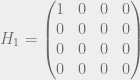
So $H_1$ is the following matrix:

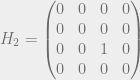
$H_1 = \begin{pmatrix} 1 & 0 & 0 & 0 \\ 0 & 0 & 0 & 0 \\ 0 & 0 & 0 & 0 \\ 0 & 0 & 0 & 0 \end{pmatrix}$

We also have

$H_2 = \begin{pmatrix} 0 & 0 & 0 & 0 \\ 0 & 0 & 0 & 0 \\ 0 & 0 & 1 & 0 \\ 0 & 0 & 0 & 0 \end{pmatrix}$

Then,
$\begin{aligned} H &= (H_1)_{1,2} \otimes I_{3} + (H_2)_{1,3} \otimes I_{2} \\ &= \begin{pmatrix} 1&&&&&&& \\ &1&&&&&& \\ &&0&&&&& \\ &&&0&&&& \\ &&&&0&&& \\ &&&&&0&& \\ &&&&&&0& \\ &&&&&&&0 \end{pmatrix} + \begin{pmatrix} 0&&&&&&& \\ &0&&&&&& \\ &&0&&&&& \\ &&&0&&&& \\ &&&&1&&& \\ &&&&&0&& \\ &&&&&&1& \\ &&&&&&&0 \end{pmatrix} \\ &= \begin{pmatrix} 1&&&&&&& \\ &1&&&&&& \\ &&0&&&&& \\ &&&0&&&& \\ &&&&1&&& \\ &&&&&0&& \\ &&&&&&1& \\ &&&&&&&0 \end{pmatrix}\end{aligned}$

$H$ has diagonal entries that are zero, so it has 0 as an eigenvalue. We can therefore conclude that $\varphi$ is satisfiable. (In this example it was easy to write out $H$ and see that it has zeros on the diagonal, but when $n$ is large, $H$ becomes exponentially big, so we can’t just compute it explicitly and look through its diagonal entries.)

Quantum Cook-Levin Theorem

We’ve seen that any $k$ -CSP problem can be thought of as a $k$ -LH problem (with a diagonal Hamiltonian matrix). And the analogy can be drawn even further. One reason $k$ -CSP is so useful is that it (and in particular 3-SAT) is NP-complete, according to the Cook-Levin Theorem. 3-SAT captures the difficulty of classical efficiently verifiable computation. It may not come as a surprise, then, that $k$ -LH captures the difficulty of quantum efficiently verifiable computation. This result is the “quantum Cook-Levin theorem”, but before we see it we need to define the complexity class QMA, the quantum analogue of NP.

Because quantum computation is probabilistic, QMA is more precisely the quantum analogue of MA (Merlin Arthur), which allows the verifier to have a chance of error:

$L \in \text{MA}$ iff there exists a probabilistic poly-time verifier $V$ and a polynomial $p(n)$ such that

$\forall x \in L, \exists y \in \{0,1\}^{p(n)},\quad \Pr[V(x,y) = 1] \geq \frac{2}{3}$
$\forall x \notin L$ , $\forall |y\rangle \in \{0,1\}^{p(n)},\quad \Pr[V(x,y) = 1] \leq \frac{1}{3}$

For QMA, the verifier is a quantum computer and the witness is a quantum state. Moreover, we’re interested in the complexity of promise problems:

QMA

A promise problem $L = L_{yes} \cup L_{no} \in \text{QMA}$ iff there exists a quantum poly-time verifier $V$ and a polynomial $p$ such that

$\forall x \in L_{yes}, \exists |y\rangle \in (\mathbb{C}^2)^{\otimes p(|x|)},\quad \Pr[V(|x\rangle|y\rangle) = 1] \geq \frac{2}{3}$
$\forall x \notin L_{no}$ , $\forall |y\rangle \in (\mathbb{C}^2)^{\otimes p(|x|)},\quad \Pr[V(|x\rangle|y\rangle) = 1] \leq \frac{1}{3}$

A problem is QMA-complete if it is in QMA and if any problem in QMA can be reduced to it in polynomial time. In 2002, Kitaev proved that $k$ -LH is QMA-complete for all $k \geq 5$ . This was the first time a natural problem was shown to be QMA-complete. In 2003 Kempe and Regev proved that 3-LH is QMA-complete, and finally in 2006 Kempe, Kitaev and Regev proved that 2-LH is QMA complete, achieving the best possible result unless P = QMA. (3-SAT is NP-complete but 2-SAT is in P, so it may seem curious that 2-LH is QMA-complete. But in fact, this isn’t too surprising, because as we mentioned earlier, $k$ -LH corresponds to MAX- $k$ -SAT, and MAX-2-SAT is NP-complete.)

“Quantum Cook-Levin Theorem”

The 2-local Hamiltonian problem is QMA-complete.

A very sketchy proof sketch. This theorem is called the quantum Cook-Levin theorem not just because of the result, but also because the proof is along the same lines as the proof of the Cook-Levin theorem.

Recall that in the proof of the Cook-Levin theorem, we start with a verifier Turing machine that takes as input $(x,y)$ and, in time $p(n)$ accepts iff $y$ is a valid witness for $x$ being in the language. We then devise (for each $n$ ) a 3-SAT formula such that any satisfying solution to the instance must be an encoding of a valid history of the Turing machine from start to finish on the input $x$ . The constraints must guarantee that (a) the input indeed starts with $x$ , (b) at every time step $t \in [1,p(n)]$ the state of the machine correctly follows from its state at time $t-1$ , and that (c) the final state of the machine indicates acceptance. The constraints for (a) and (c) are trivial, and the reason we can do (b) is because Turing machines compute locally.

For our quantum Cook-Levin proof, we follow the same template. Given a quantum circuit, we construct a local Hamiltonian that has ground energy below some constant only if there is a quantum encoding of the circuit that includes the proper (a) initial state, (b) intermediate computation, and (c) final state. As before, (a) and (c) are easy, because the parts of the initial and final states we need to ‘inspect’ (with the local terms of the Hamiltonian) are essentially classical. But when we try to compute local constraints for (b), we run into a big problem: entanglement.

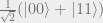
Consider some step of the computation. This will consist of applying a quantum gate $U$ to a state $|\psi\rangle$ to obtain $|\psi'\rangle = U|\psi\rangle$ . Even assuming we’ve already written down constraints to verify that $|\psi\rangle$ is correct, it is non-trivial to write down constraints to verify that $|\psi'\rangle = U|\psi\rangle$ because $|\psi'\rangle$ may differ from $U|\psi\rangle$ in a highly non-local way if there is entanglement between far-flung qubits. For example, suppose for the sake of illustration that $|\psi\rangle = \frac{1}{\sqrt{2}}(|00\rangle + |11\rangle)$ and $U = I$ . And suppose we want to check that $|\psi'\rangle = \frac{1}{\sqrt{2}}(|00\rangle + |11\rangle)$ with 1-local constraints. Unfortunately, there is no way to distinguish $\frac{1}{\sqrt{2}}(|00\rangle + |11\rangle)$ from $\frac{1}{\sqrt{2}}(|00\rangle - |11\rangle)$ by looking at one qubit at a time: the reduced density matrix of either state for either qubit is the same: $I$ /2. There are examples like this that apply for $k$ -local constraints for any $k >1$ , so we can’t even verify the ‘trivial’ gate $I$ , let alone gates that actually change the state. It would seem that we are stuck.

Luckily, although quantum superposition makes this problem more difficult, we can actually use superposition in a clever manner in order to surmount the difficulty. Instead of encoding the states $|\psi\rangle$ and $|\psi'\rangle$ separately, we can put them in superposition in a way that will allow us to verify that $|\psi'\rangle = U|\psi\rangle$ . Suppose again that $U = I$ , so we want to check that $|\psi'\rangle = |\psi\rangle$ . Let $|\eta\rangle = \frac{1}{\sqrt{2}}(|\psi\rangle|0\rangle + |\psi'\rangle|1\rangle)$ . Then, just by looking at the last qubit of $|\eta\rangle$ , we can tell how close $|\psi'\rangle$ is to $|\psi\rangle$ : the reduced density matrix of the last qubit contains information about the angle between $|\psi\rangle$ and $|\psi'\rangle$ :

$\begin{pmatrix} 1 & \langle\psi|\psi'\rangle \\ \langle\psi|\psi'\rangle & 1 \end{pmatrix}$

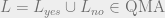
The challenge is to describe a $k$ -local Hamiltonian $H$ that has a state with energy below some parameter $a$ whenever $y$ is a valid witness for $x$ , and otherwise has no state with energy below $b>a$ . We won’t cover the details here, but the crucial idea is that when $y$ is a valid witness for $x$ , the following ‘witness state’ (which is a superposition of the states of the quantum computer over all the time steps) will have low energy for a carefully-devised $H$ :

$|\eta\rangle = \frac{1}{p(n)}\sum_{t=0}^{p(n)}(U_t\cdots U_1|\psi_0\rangle)\otimes|t\rangle$

where $|\psi_0\rangle = |x\rangle|y\rangle|0\rangle^{\otimes m}$ is the initial state of the computation, and $|t\rangle$ is called the “clock register”. Note that because the size of the clock register is logarithmic in $n$ , we actually need to use $\log(n)$ -local constraints. For 5-local constraints to suffice, the witness state will need to be a little more complicated (the proof for 2-local constraints is even more difficult). Even for the case of $\log(n)$ -LH, the complete proof must demonstrate that no state besides the witness state has low energy.

□

Roadmap

The upshot is that 2-LH is the canonical QMA-complete problem. This is a beautiful result from a quantum complexity theory perspective, but from a physics perspective it is very bad news. The QMA-completeness of the local Hamiltonian problem means that (presuming BQP $\neq$ QMA) we can’t solve 2-LH, and we couldn’t even solve it with a quantum computer. Because of the central importance of finding the ground energy, this in turn means that almost anything a physicist would like to compute about a system is intractable.

So is all hope lost? No! Just as we started out wanting to understand Hamiltonians in general and restricted our focus to local Hamiltonians, the approach the physics community has taken is to focus on even more restricted classes of Hamiltonians that still capture interesting physical systems. One route is to restrict the topology of the system encoded by the Hamiltonian: for example, in many physics models, the particles form a low-dimensional lattice and the only interactions between them are 2-local interactions along edges. Even this isn’t enough, though: the problem remains QMA-hard on many simple topologies like lattices (for example, 2-LH on the 2-D lattice is QMA-complete, and 2-LH on even the 1-D lattice is QMA-complete when instead of qubits we are dealing with 8-dimensional qudits). So we add a further restriction, which is to focus on gapped Hamiltonians: these are Hamiltonians for which there is a constant gap between the ground energy and the second-lowest energy.

Even local Hamiltonians are intractable in general. Gapped Hamiltonians on low-dimensional lattices, though, may be tractable.

Thus, in the notes to follow, we will focus our energies on trying to solve the gapped local Hamiltonian problem for 1-D and 2-D lattices. The reason there is hope in these settings is that entanglement is (or is conjectured to be) limited by ‘area laws’. In the next post, Fred Zhang will describe a diagrammatic language (‘tensor networks’) for thinking about low-entanglement quantum states, and he’ll show how physicists solve the local Hamiltonian problem for gapped 1-D systems.

3 thoughts on “What is Quantum Hamiltonian Complexity?”

Pingback: Tensor Networks, Matrix Product States and Density Matrix Renormalization Group | Windows On Theory
Pingback: A 1D Area Law for Gapped Local Hamiltonians | Windows On Theory
Pingback: Towards Quantum PCP: A Proof of the NLETS Theorem | Windows On Theory

	Interview about this… on Men in Computer Science
	Interview about this… on The Swiss Army Knife of C…
	Interview about this… on An alarming trend in K-12 Math…
	Interview about this… on The uneasy relationship betwee…
	Interview about this… on The different forms of quantum…

What is Quantum Hamiltonian Complexity?

Classical energy and ground states

Quantum Hamiltonians

The Local Hamiltonian problem

Computer science motivation

Quantum Cook-Levin Theorem

Roadmap

Published by benedelman

3 thoughts on “What is Quantum Hamiltonian Complexity?”

Leave a Reply Cancel reply

Classical energy and ground states

Quantum Hamiltonians

The Local Hamiltonian problem

Computer science motivation

Quantum Cook-Levin Theorem

Roadmap

Share this:

Like this:

Related

Published by benedelman

3 thoughts on “What is Quantum Hamiltonian Complexity?”

Leave a Reply Cancel reply