(This post is based on part of a lecture delivered by Boriana Gjura and Prayaag Venkat. See also posts by Ben Edelman and Fred Zhang for more context on Quantum Hamiltonian Complexity.)

Introduction

In this post we present the Area Law conjecture and prove it rigorously,
emphasizing the emergence of approximate ground state projectors as a
useful and promising tool.

The difficulty of understanding many-body physics lies in this dichotomy
between the power of quantum on the one hand, and the fact that even
describing a quantum state requires exponential resources on the other.
A natural way to proceed is to ask if the special class of physically
relevant states admits succinct descriptions. As seen in a previous
post, the QMA-completenes of the $k$ -local Hamiltonian problem suggests
that even ground states of local Hamiltonians do not admit such
descriptions. Looking at these ground states, the following questions
arise naturally.

When do the ground states of local Hamiltonians have a special
structure? When does that structure allow for a meaningful short
description? When does that structure allow us to compute properties
of them?

As stated informally, the answer to these questions is yes for (gapped)
1D systems, and it is an open problem to answer these in higher
dimensions.

The Area Law

The Area Law is inspired by the Holographic principle in Cosmology,
which informally states that the total information in a black hole
resides on the boundary. That is, the complexity of the system depends
on the size of its boundary, not its volume.

Preliminaries

For the sake of clarity, we assume that $H = \sum_{i=1}^m H_i$ is a
2-local Hamiltonian on qubits, each $0 \leq \| H_i \| \leq 1$ is a
projection $(H_i^2 = H_i)$ , $H$ is frustration free, (meaning that
$\lambda_0(H)$ , the lowest eigenvalue, is zero) and there is a unique
ground state $| \psi_0 \rangle$ .

These conditions simplify our proof. It will be easy to generalize to
$0 \leq \| H_i \| \leq 1$ and relaxing to $q$ -local on qudits (dimension
$d$ particles). The most significant assumption is that $H$ is
frustration-free: more work is necessary to make the proof work
otherwise.

To formalize our conjecture, we define a notion of von Neumman entropy
below.

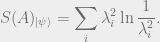
Definition: Consider any state $| \psi \rangle$ lying in a bipartite Hilbert space
$\mathcal{H}_A \otimes \mathcal{H}_B$ , and perform a Schmidt
decomposition to obtain
$| \psi \rangle = \sum_{i =1}^{d} \lambda_i | u_i \rangle_A| v_i \rangle_B$ .
The Von Neumann entanglement entropy of $| \psi \rangle$ across region A
is defined as
$\displaystyle S(A)_{| \psi \rangle} = \sum_i \lambda_i^2 \ln \frac{1}{\lambda_i^2}.$

Why is this a good notion of entropy? If
$| \psi \rangle = | L \rangle \otimes | R \rangle$ , then
$S_{| \psi \rangle} = 0$ , i.e. the product state has no entanglement. On
the other hand, the maximally entangled state
$| \psi \rangle = \sum_{i = 1}^D \frac{1}{\sqrt{D}} | i \rangle_A \otimes | i \rangle_B$
has entropy $S_{| \psi \rangle} = \ln(D)$ . In general, we have that

$\displaystyle S_{| \psi \rangle} \leq \ln(\dim \text{Hilbert space}).$
This is a
direct quantum generalization of the fact that a classical probability
distribution on $D$ elements has entropy at most $\ln D$ , and this is
achieved by the uniform distribution.\
We can now state the Area Law.

Conjecture: Let $| \psi_0 \rangle$ be the ground state of $H$ , as defined above.
Then for any region $A$ (i.e. a subset of qubits),

$\displaystyle S_{| \psi_0 \rangle} \leq \ln (\dim \partial A),$
where $\partial A$
denotes the boundary of the region $A$ , the set of qubits that interact
through $H$ with at least a qubit outside of region $A$ .

This conjecture is illustrated by the following figure.

area2
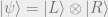
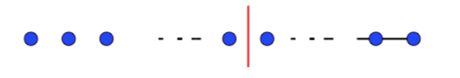
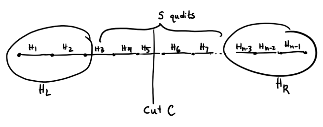
We prove the 1-D version of this conjecture. Note that for a 1D system
(i.e. qubits on a line with nearest neighbor interactions) it suffices
to consider bipartitions of the Hilbert space defined by a “cut” (see
the figure below). By a cut, we mean a partition of the qubits into two
sets consisting of all the qubits to the left and right, respectively,
of a fixed qubit $i^*$ .

area1

Theorem: Let $| \psi_0 \rangle$ be as above. Then for any cut $C = (i^*, i^*+1)$ ,
$\displaystyle S(C)_{| \psi_0 \rangle} \leq O(1).$

Approximate Ground State Projectors

In the case where all $H_i$ commute, consider the operator
$A = \prod_i (I - H_i)$ . This operator will project any product state
onto the ground state. Therefore, we can get a representation of the
ground state as a matrix product state (as we saw in a previous post on
tensor networks). Can we generalize this idea when the $H_i$ do not
necessarily commute?

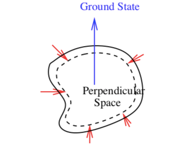
A natural idea is to define an operator that approximately projects a
state onto the vector we want (the ground state), while shrinking it on
the other directions. We also want this operator to not increase
entanglement too much. The proof of the area law will involve
constructing a low-rank tensor approximate factorization of the ground
state by starting with a factorized state, which has a good overlap with
the ground state, and then repeatedly applying such an operator.

agsp

We first give a formal definition of an approximate ground state
projector. In the following, under the assumption of the existence of
such an object, we will prove the area law. At the end, we will show how
to construct it.

Definition: $K$ is a $(D,\Delta)$ –approximate ground state projection (AGSP) if:
1. $K | \psi_0 \rangle = | \psi_0 \rangle$
2. For every $| \Gamma \rangle$ such that
$\langle \Gamma | \psi_0 \rangle = 0$ , then
$\| K | \Gamma \rangle \|^2 \leq \Delta \| | \Gamma \rangle \|^2$ .
3. $K$ has entanglement rank at most $D$ . That is, $K$ admits a Schmidt
decomposition of the form $K = \sum_{i=1}^{D} L_i \otimes R_i$ ,
where $L_i$ and $R_i$ act only on the particles to the left and
right of the cut, respectively.

The first step of the proof of the Area Law is to find a product state
that has a good overlap with the ground state. That is, it should have a
constant overlap that is not dependent on $n$ , the number of particles
in the system.

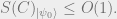
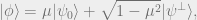
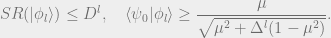
Lemma 1: Suppose there exists a $(D, \Delta)$ -AGSP such that
$D \Delta \leq \frac{1}{2}$ . Fix a partition $(A, \bar{A})$ of the space
on which the Hamiltonian acts. Then there exists a product state
$| \phi \rangle = | L \rangle_A \otimes | R \rangle_{\bar{A}}$ such that
$\displaystyle \langle \phi | \psi_0 \rangle = \mu \geq \frac{1}{\sqrt{2D}}$

Proof:
Let $| \phi \rangle$ be a product state with the largest overlap in
$| \psi_0 \rangle$ , meaning that it maximizes.
$\langle \phi | \psi_0 \rangle = \mu$ and can be written as
$\displaystyle | \phi \rangle = \mu | \psi_0 \rangle + \sqrt{1 - \mu^2} | \psi^{\perp} \rangle,$
where the latter is some state orthogonal to the ground state. We apply
$K$ to get
$\displaystyle K | \phi \rangle = \mu | \psi_0 \rangle + \delta | \psi' \rangle$
where $|\delta|^2 \leq \Delta$ and $| \psi' \rangle$ is normalized. By
the properties of the operator $K$ , the decomposition of
$K | \psi_0 \rangle$ has at most $D$ terms. Using the Cauchy-Schwarz
inequality:
$\displaystyle \begin{aligned} \mu = \big| \sum_i \lambda_i \langle \psi_0 | | L \rangle_i | R \rangle_i\big| &\leq \sqrt{\sum_i \lambda_i ^2} \sqrt{\langle \psi_0 | | L \rangle_i | R \rangle_i^2} \\ &\leq \sqrt{\mu^2 + \Delta} \sqrt{D} \sqrt{\max_i \langle \psi_0 | | L \rangle_i | R \rangle_i}\end{aligned}$

Therefore there exists a product state such that
$\mu \geq | \langle \psi_0 | | L \rangle_i | R \rangle_i| \geq \frac{\mu}{\sqrt{D(\mu^2 +D)}}$ ,
which implies that $\mu^2 \geq \frac{1}{2D}$ , as desired. $\Box$

Starting with a product state with a big enough overlap with the ground
state, the proof of the next lemma shows how we can repeatedly apply
AGSPs to bound the entropy across the cut.

Lemma 2: Suppose there exists a $(D, \Delta)$ -AGSP such that
$D \Delta \leq \frac{1}{2}$ , and a product state
$| \phi \rangle = | L \rangle_A \otimes | R \rangle_{\bar{A}}$ such that
$\langle \phi | \psi_o \rangle = \mu$ . Then
$\displaystyle S_{| \psi_0 \rangle} \leq O(1) \frac{\log \mu}{\log \Delta} \log{D}$

But before we prove this, let’s state an intuitive result of Eckart and
Young, which provides an upper bound for the overlap of two states given
the Schmidt rank of one.

Lemma (Eckart-Young): Let $| \psi \rangle \in L \otimes R$ be a normalized
vector with Schmidt decomposition
$| \psi \rangle = \sum_i \lambda_i | u_i \rangle| v_i \rangle$ , where
$\lambda_1 \geq \lambda_2 \geq \dots$ . Then for any normalized
$| \phi \rangle \in L \otimes R$ it holds that
$\displaystyle | \langle \psi | \phi \rangle| \leq \sqrt{\sum_{i} \lambda_i^2}$

Using this result, we continue the proof.

Proof of Lemma 2:
Write the $(D, \Delta)$ -AGSP as $K$ . Given a state $| \phi \rangle$ , we
denote by $| \phi_l \rangle$ the normalized stated after applying $l$
projections on the state, namely
$\displaystyle | \phi_l \rangle = \frac{K^l | \phi \rangle}{\|K^l | \phi \rangle\|}.$
By the way we’ve defined $K$ , the Schmidt rank of $| \phi_l \rangle$
increases by a power of $l$ , and this state has an improved overlap with
the ground state, that is:
$\displaystyle SR(| \phi_l \rangle) \leq D^l, \quad \langle \psi_0 | \phi_l \rangle \geq \frac{\mu}{\sqrt{\mu^2 + \Delta^l(1 - \mu^2)}}.$

Let $| \psi_0 \rangle = \sum_i \lambda_i | L_i \rangle| R_i \rangle$ be
the Schmidt decomposition of the ground state relative to the cut
$(i^*, i^*+1)$ , where $\lambda_1 \geq \lambda_2 \geq \dots$ . The
Eckart-Young theorem gives:
$\displaystyle \sum_{i=1}^{D^l} \lambda_i^2 \geq | \langle \psi_0 | \phi_l \rangle|^2 \geq \frac{\mu^2}{\mu^2 + \Delta^l (1 - \mu^2)}$
from which
$\displaystyle \sum_{i> D^l} \lambda_i^2 \leq 1 - \frac{\mu^2}{\mu^2 + \Delta^l (1 - \mu^2)} \leq \frac{\Delta^l}{\mu^2}$

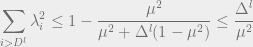
We choose
$l_0 = 2 \frac{\log \mu}{\log \Delta} - \frac{\log 2}{\log \Delta}$ such
that $\frac{\Delta^{l_0}}{\mu^2} \leq \frac{1}{2}$ . Let’s now bound the
worst case entropy accross the AGSP cut. The first $D^{l_0}$ Schmidt
coefficients account for an entropy of at most $l_0 \log D$ . For the
remaining coefficients, we group them in chunks of size $D^{l_0}$ in
intervals $[D^{kl_0} + 1, D^{(k+1)l_0}]$ indexed by $k$ . For each of
these intervals, the corresponding entropy can be upper bounded by
$\displaystyle \frac{\delta^{kl_0}}{\mu^2} \log D^{(k+1)l_0} = l_0 \frac{1}{2^k} (k+1) \log D$
where here $\frac{\Delta^{kl_0}}{\mu^2}$ is an upper bound on the total
probability mass in the interval, and $D^{-(k+1)l_0}$ a lower bound on
the size of any Schmidt coefficient (squared) in the interval. This
follows from the fact that they are organized in descending order and
must sum to 1.

Therefore, the total entropy is
$\displaystyle \begin{aligned} S((i^* ,i^* +1)) &\leq l_0 \log D + \sum_{k \geq 1} l_0\frac{1}{2^k}(k+1) \log D \\ &\leq l_0 \log D + l_0 \log D \sum_{k \geq 1} \frac{1}{2^k}(k+1) \\ &\leq O(1) l_0 \log D \\ &\leq O(1) \frac{\log \mu}{\log \Delta}\log D\end{aligned}$

This bound depends on $D$ and $\Delta$ . This is sufficient to imply the
Area Law because our AGSP constructions will have constant $D$ and
$\Delta$ . $\Box$

AGSP Construction

In this section, our goal is to construct an AGSP with the correct
tradeoff in parameters. We briefly recall the intuition behind the
properties that an AGSP must satisfy. First, the AGSP should leave the
ground state untouched. Second, it shrinks states which are orthogonal
to the fround state. Third, it should not increase the entanglement
across the cut by too much (see the figure below).

A depiction of the third property in the AGSP definition for a 1D
system. The property that $K$ is a sum of tensor products of operators
which only act on one “side” of the
system.

schmidt-rank
We are interested in understanding a construction of an AGSP for three
reasons:

As we saw before, we can prove a 1D area law assuming the existence
of an AGSP with good parameters.
AGSPs have been used a building block in an provably polynomial-time
algorithm for finding ground states of gapped 1D local Hamiltonians.
They appear to be a general purpose tool with potential applications
in other contexts.

Details of the construction

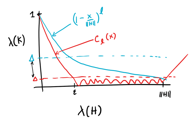
One way to think about the the first two properties in the AGSP
definition is in terms of the relationship of the eigenvalues of $K$ and
the eigenvalues of $H$ (see the figure below). The first property says
that the ground state of $H$ should be an eigenvector of $K$ with
eigenvalue 1. The second property says that all other eigenvectors of
$H$ should be mapped to eigenvectors of $K$ with eigenvalue at most
$\sqrt{\Delta}$ .

In this plot, the horizontal axis represents the eigenvalues of $H$
and the vertical axis represents the eigenvalues of $K$ . The ground
state of $H$ , which corresponds to the eigenvalue 0, should remain fixed
upon applying $K$ to
it.

spectrum-plot
In the following, we will aim to construct and AGSP whose tradeoff in
parameters allows us to achieve the following result.

Theorem: $S_{| \psi_0 \rangle}(A) = O(\frac{\log^2 d}{\epsilon})$ .

Attempt 1

As a first attempt, we will evaluate the quality of the following
operator:
$\displaystyle K = (1-\frac{H}{\| H \|})^l,$
where $l$ is some natural
number that we will decide upon later. We now check the three properties
for this particular choice of $K$ .

First, it is clear that $K$ does not change the ground state, since the
ground state is an eigenvector of $H$ with eigenvalue 0
(frustration-free case). Second, because any other eigenvalue of $H$ is
at least $\epsilon$ (the energy gap), we have that
$\Delta \leq (1-\frac{\epsilon}{\| H \|})^l \approx e^{-\frac{\epsilon}{\| H \|} l}$ .
Third, for the time being, let us think of $l$ as roughly corresponding
to $D$ (we will formalize this later).

Unfortunately, these values $\Delta$ and $D$ will not allow us to
achieve the desired tradeoff of $D \Delta \leq \frac{1}{2}$ . To see why
this is, observe that because we have $n-1$ local Hamiltonians, the term
$\| H \|$ could be on the order of $n$ (recall that
$0 \leq \| H_i \| \leq 1$ ), so we would need to choose $l$ proportional
to $n$ to reduce $\Delta$ to a constant (see figure below). Unfortunately, this will result in a
corresponding increase in $D$ , violating $D \Delta \leq \frac{1}{2}$ .

The first attempt an AGSP corresponds to the polynomial is depicted in
blue. This polynomial does not decay at a fast enough rate, so the
second attempt will replace it with another polynomials, depicted in
red, which decays much
faster.

polynomials

Attempt 2

In summary, the two weaknesses of the previous approach we need to
address are:

The large $\| H \|$ term in the exponent substantially reduces the
shinking effect of applying the AGSP. We will address this using the
technique of Hamiltonian truncation.
For a fixed $l$ (roughly corresponding to the entanglement rank of
$K$ ), the function $f(x) = (1 - \frac{x}{\| H \|})^l$ does not decay
fast enough after the point $x = 0$ (which is the ground state
energy). We will address this using Chebyshev polynomials.

As discussed before, the $\| H \|$ term is large because it involves
contribution from all $n-1$ local Hamiltonians. Intuitively, we might
believe that only the local Hamiltonians near the site of the cut itself
should play a large role in the entanglement of the ground state across
the cut. Specifically, if we write
$H = H_1 + \ldots H_{n-1} = H_L + H_{i_1} + \ldots H_{i_s} + H_R$ , where
$H_{i_j}$ are the $s$ local Hamiltonians neighboring the cut and $H_L$
and $H_R$ are the “aggregrated” Hamiltonians of all the remaining local
Hamiltonians to the left and right, respectively, of $H_{i_1}$ and
$H_{i_s}$ , then we are asserting that $H_L$ and $H_R$ contribute
significantly to $\| H \|$ but are not important when trying to
characterize the ground state (see figure below).

We keep track of the local Hamiltonians corresponding to the $s$
qudits directly surrounding the cut. The remaining local Hamiltonians
are aggregated into the Hamiltonians $H_L$ and $H_R$ , whose eigenvalues
will be truncated to define
$H'$ .

truncation
Mathematically, if we let
$H' = H^{\leq t}_L + H_{i_1} + \ldots H_{i_s} + H^{\leq t}_R$ , where
$H^{\leq t}_i$ denotes operator obtained by truncating all eigenvalues
of $H$ to be at most $t$ , we claim the following:

Claim:
1. $\| H' \| \leq s + 2t$
2. $| \psi_0 \rangle$ is a ground state of $H'$ .
3. $H'$ has gap $\epsilon' = \Omega (\epsilon)$

It is straightforward to verify the two first two claims, We omit the
proof of the third claim. Intuitively, we have chosen $H'$ to be an
approximation of $H$ which has much smaller norm.

Next, we come to the task of designing a degree- $l$ polynomial $p$ which
decays faster than our first attempt $f(x) = (1 - \frac{x}{\| H \|})^l$
after the point $x=0$ . In other words, we would like $p$ to satisfy
$p(0) = 1$ (fixing the ground energy) and map the interval
$[\epsilon, \| H' \|]$ to the interval $[0,\Delta]$ for as small a
$\Delta$ as possible. It turns out that the degree- $l$ Chebyshev
polynomial (of the first kind) is precisely the polynomial which has
this behavior (see the appendix for a review of Chebyshev polynomials).
Letting $T_l$ denote the degree- $l$ Chebyshev polynomial, we take our
polynomial to be a scaled and shifted version of it:
$\displaystyle p(x) = T_l\left(\frac{\| H' \| + \epsilon' - 2x}{\| H' \| - \epsilon'}\right)/T_l\left(\frac{\| H' \| + \epsilon'}{\| H' \| - \epsilon'}\right)$
Given this definition of $p$ , we take our new candidate AGSP to be
$K = p(H)$ , which has the following guarantees:

Claim:
1. $K | \psi_0 \rangle = | \psi_0 \rangle$
2. $K$ achieves
$\Delta = O(\exp{-\sqrt{\frac{\epsilon'}{\| H' \|}} l})$
3. $K$ achieves $D = O(d^{\frac{l}{s} + s})$

The first claim is straightforward to verify. The proof of the second
claim is ommitted; it involves calculations making use of standard
properties of Chebyshev polynomials. We remark that the dependence of
the exponent $\Delta$ on $\| H' \|$ has been reduced by a quadratic
amount, compared with the first attempt at an AGSP. We now sketch the
main ideas behind the proof of the third claim. After that, we will
choose values of $s$ and $t$ so that the desired tradeoff $D \Delta$ is
achieved.

We have defined $K$ as a degree- $l$ polynomial in $H'$ , so we may write
it as: $\displaystyle K = \sum_{j=0}^{l} c_i (H')^j,$ where $c_i$ are coefficients
whose particular values are not relevant to the analysis of the Schmidt
rank of $K$ across the given cut. It is straightforward to check that
the Schmidt rank of $K$ is bounded by the sum of the ranks of the
monomials $(H')^j$ (subadditivity). So, it suffices to analyze the
Schmidt rank of the monomial of the largest degree, $(H')^l$ .

From our expression for $H'$ , we can expand this power to get:
$\displaystyle (H')^l = (H^{\leq t}_L + H_{j_1} + \ldots H_{j_s} + H^{\leq t}_R)^l = \sum_{j_1,\ldots,j_l} H_{j_1} \cdots H_{j_l},$
where the summation is over all products of $l$ Hamiltonians from the
set $\{H^{\leq t}_L, H_{i_1}, \ldots H_{i_s}, H^{\leq t}_R\}$ . Now, one
natural approach to proceed is to analyze the Schmidt rank of each term
in the summation, and then sum over all the terms. Unfortunately, this
approach will not work because there are exponentially many terms in the
summation, so our estimate of $D$ will be too large. To address this
issue, it is possible to collect terms cleverly so that the total number
of terms is small. However, we will not provide the details here; we
will just sketch how analyze the Schmidt rank of an individual term.

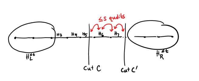
The term $H_{j_1} \cdots H_{j_l}$ consists of a product of $l$
Hamiltonians. Since there are $s+1$ possible locations of a cut that is
crossed by one of the $H_{j_k}$ , an average cut will have
$\frac{l}{s+1}$ of the $H_{j_k}$ crossing it. For each Hamiltonian which
crosses this average cut, the Schmidt rank will be multiplied by a
factor of $d^2$ . Hence, the Schmidt rank of the term
$H_{j_1} \cdots H_{j_l}$ is $O(d^\frac{2l}{s})$ . This bound on the
Schmidt rank is for an average cut $C'$ , not necessarily the cut $C$ we
fixed in the beginning. The two cuts are separated by at most $O(s)$
qudits because $C'$ is one of the $s+1$ cuts surrouding $C$ (see figure
below), so one can relate the Schmidt rank across these two cuts. For
each Hamiltonian between the two cuts, the high-level idea is that the
entanglement rank is multiplied by at most a factor of $d$ . Because the
entanglement rank across $C'$ is $O(d^\frac{2l}{s})$ , the entanglement
rank across $C$ is $O(d^{\frac{2l}{s} + s})$ .

The entanglement across cut $C$ is analyzed bounding the entanglement
across a nearby cut $C'$ and then relating the
two.

cut-to-avg-cut-D
Putting all the pieces together, we have that:

By Hamiltonian truncation and the Chebyshev polynomial construction,
$\Delta = O(e^{-l/ \sqrt{s}})$ .
By the entanglement rank analysis, $D = O(d^{\frac{l}{s} + s})$ .

One can now check that if we set $l = O(s^2)$ and
$s = O(\frac{\log^2 d}{\epsilon})$ (where large enough constants are
hidden inside the $O(\cdot)$ ), then we achieve the desired tradeoff of
$D \Delta \leq \frac{1}{2}$ . Note that $l$ and $s$ are constants because
$d$ and $\epsilon$ are constants.

Towards an area law in high dimensions

One of the major open problems in this line of work is to prove an area
law for 2D systems. We now discuss one potential line of attack on this
problem, based on a reduction to the 1D area law we have proven using
AGSPs.

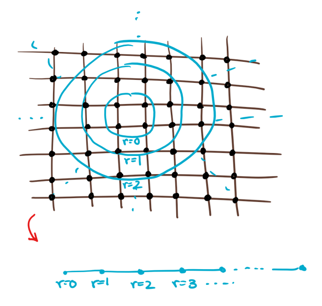
Consider a 2D system, as depicted in the figure below. We can form a
sequence of concentric shells of qudits of increasing radii and
“contract” each shell into a single qudit of higher dimension. That is,
if each of the original qudits have dimension $d$ and we consider the
shell at radius $r$ , the dimension of the contracted qudit is roughly
$d^r$ because there are roughly $r$ qudits in the shell. The system of
contracted qudits is now a 1D system in the sense that the shell at
radius $r$ only interacts with the shells at radii $r-1$ and $r+1$ .

A 2D system can be reduced to a 1D system by decomposing it into a
sequence of concentric
“shells”.

two-dim-area-law
Suppose that we were able to show an area law as discussed previously,
but with the following dependence on $d$ :

$\displaystyle S_{| \psi_0 \rangle}(A) = O(\frac{\log d}{\epsilon}).$
If we replace
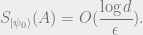
$d$ with $d^r$ , the dimensionality in our new 1D system, we get that

$\displaystyle S_{| \psi_0 \rangle}(A) = O(\frac{r}{\epsilon}),$
which is exactly an
area law in 2D (recalling that surface area of a circle is proportional
to its radius). In fact, even the weaker result of proving that
$S_{| \psi_0 \rangle}(A) = O(\frac{\log^{2-\alpha} d}{\epsilon})$ for
some $\alpha > 0$ would imply a “sub-volume law”, already a major
breakthrough. This suggests that constructing AGSPs with better
parameters may be a plausible approach to proving an area law.

Future Directions

In addition to proving an area law in 2D, there are several interesting
questions raised by what we discussed here. See the survey of Gharibian
et al. for more details.

Do area laws hold for gapless (i.e. non-constant gap, or “critical”)
systems? No, there are known counterexamples.
Do area laws hold for degenerate systems (where the ground state is
not unique)? Yes, the AGSP approach still works for systems with
groundspaces of constant dimension. It is unknown whether area laws
hold when the groundspace is of dimension polynomial in $n$ .
Can one design practical algorithms for finding ground states of
gapped 1D local Hamiltonians? Yes, there is one approach based on
AGSPs.
Do area laws hold in general for systems where the interactions are
not necessarily described by a lattice? No, there are known
counterexamples to such a “generalized area law”?

Acknowledgements

We would like to thank Boaz Barak and Tselil Schramm for their guidance
in preparing the talk on which this post is based.

Most of this post (including some figures) draws heavily upon the
following resources: lecture notes from courses taught by Thomas Vidick and Umesh Vazirani,
repectively, and a survey by Gharibian et al.
In these notes, we have opted to illustrate the main ideas, while
glossing over technical details. Our goal with this approach is to
prepare the reader to more easily understand the original sources and
highlight the some of the key concepts.

Appendix: Background on Chebyshev Polynomials

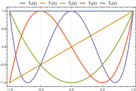
The Chebsyhev polynomials $\{T_l\}_{l \in \mathbb{N}}$ are a family of
polynomials with many special properties. They are defined as
$T_0(x) = 1$ , $T_1(x) = x$ and $\displaystyle T_l(x) = 2xT_{l-1}(x) - T_{l-2}(x).$
The first few polynomials are plotted below (Source:
<https://en.wikipedia.org/wiki/Chebyshev_polynomials>).

chebyshevs
Below, we state a property (proof ommitted) which provides some
intuition as to why Chebyshev polynomials are the “correct” choice for
our construction. Intuitively, it says that among all degree- $l$
polynomials which are trapped inside $[-1,1]$ on the interval $[-1,1]$ ,
$T_l$ dominates $p$ outside of $[-1,1]$ .

Claim: Let $p: \mathbb{R} \rightarrow \mathbb{R}$ be a degree- $l$ polynomial
such that $|p(x)| \leq 1$ for all $x \in [-1,1]$ . Then for all
$|x| \geq 1$ , $|p(x)| \leq |T_l(x)|$ .

References

Sevag Gharibian, Yichen Huang, Zeph Landau, Seung Woo Shin, et al. “Quantum Hamiltonian Complexity”. Foundations and Trends in Theoretical Computer Science, 10(3):159–282, 2015.
Thomas Vidick. Lecture notes for CS286 seminar in computer science: “Around the quantum PCP conjecture”. http://users.cms.caltech.edu/~vidick/teaching/286_qPCP/index.html, Fall 2014.
Umesh Vazirani. Lecture notes for CS294-4 “Quantum computation”. https://people.eecs.berkeley.edu/~vazirani/f16quantum.html, Fall 2016.

	Mostafa Touny on Avi wins the Turing, TCS for…
	Harvard Professors o… on Open letter to the Harvard…
	Harvard Professors o… on Open letter to the Harvard…
	Harvard, we have a p… on Letter to the Harvard Corporat…
	Eitan bachmat on Letter to the Harvard Corporat…

A 1D Area Law for Gapped Local Hamiltonians

Introduction

The Area Law

Preliminaries

Approximate Ground State Projectors

AGSP Construction

Details of the construction

Attempt 1

Attempt 2

Towards an area law in high dimensions

Future Directions

Acknowledgements

Appendix: Background on Chebyshev Polynomials

References

Published by prayaagvenkat

3 thoughts on “A 1D Area Law for Gapped Local Hamiltonians”

Leave a comment Cancel reply

Introduction

The Area Law

Preliminaries

Approximate Ground State Projectors

AGSP Construction

Details of the construction

Attempt 1

Attempt 2

Towards an area law in high dimensions

Future Directions

Acknowledgements

Appendix: Background on Chebyshev Polynomials

References

Share this:

Related

Published by prayaagvenkat

3 thoughts on “A 1D Area Law for Gapped Local Hamiltonians”

Leave a comment Cancel reply