Tensor Networks, Matrix Product States and Density Matrix Renormalization Group

by Fred Zhang

This is the second installment of a three-part series of posts on quantum Hamiltonian complexity based on lectures given by the authors in Boaz and Tselil’s seminar. For the basic definitions of local Hamiltonians, see Ben’s first post. Also check out Boriana and Prayaag’s followup note on area laws.

This post introduces tensor networks and matrix product states (MPS). These are useful linear-algebraic objects for describing quantum states of low entanglement.

We then discuss how to efficiently compute the ground states of the Hamiltonians of ${1}$ D quantum systems (using classical computers). The density matrix renormalization group (DMRG), due to White (1992, 1993), is arguably the most successful heuristic for this problem. We describe it in the language of tensor networks and MPS.

1. Introduction

We are interested in computing the ground state—the minimum eigenvector—of a quantum Hamiltonian, a $2^n \times 2^n$ complex matrix that governs the evolution of a quantum system of $n$ qubits. We restrict our attention to the local Hamiltonian, where the matrix is a sum of Hamiltonians each acting only on $k$ qubits. In the previous article, we discussed some hardness results. Namely, a local Hamiltonian can be used to encode SAT instances, and we further gave a proof that computing the ground state is QMA-Complete.

Despite the hardness results, physicists have come up with a variety of heuristics for solving this problem. If quantum interactions occur locally, we would hope that its ground state has low entanglement and thus admits a succinct classical representation. Further, we hope to find such a representation efficiently, using classical computers.

In this note, we will see tensor networks and matrix product states that formalize the idea of succinctly representing quantum states of low entanglement. As a side remark for the theoretical computer scientists here, one motivation to study tensor network is that it provides a powerful visual tool for thinking about linear algebra. It turns indices into edges in a graph and summations over indices into contractions of edges. In particular, we will soon see that the most useful inequality in TCS and mathematics can be drawn as a cute tensor network.

In the end, we will discuss the density matrix renormalization group (DMRG), which has established itself as “the most powerful tool for treating 1D quantum systems” over the last decade [FSW07]. For many 1D systems that arise from practice, the heuristic efficiently finds an (approximate) ground state in its matrix product state, specified only by a small number of parameters.

2. Tensor Networks

Now let us discuss our first subject, tensor networks. If you have not seen tensors before, it is a generalization of matrices. In computer scientists’ language, a matrix is a two-dimensional array, and a tensor is a multi-dimensional array. In other words, if we think of a matrix as a square, then a 3 dimensional tensor looks like a cube. Formally, a (complex) n dimensional tensor ${T}$ maps $n$ indices to complex values, namely, to its entries:

$\displaystyle T : [d_1] \times [d_2] \times \cdots \times [d_n] \rightarrow \mathbb{C}.$

The simplest tensor network is a graphical notation for a tensor. For an ${n}$ -dimensional tensor ${T}$ , we draw a star graph and label the center as ${T}$ and the edges as the indices. To evaluate this tensor network, we put values on the edges, i.e., indices, and then the tensor network would spit out its entry specified by the indices.

Evaluating a simple tensor network, ${T(1,5,3,1)=1/\sqrt{2}}$ . The numbers are chosen arbitrarily.

Evaluating a simple tensor network, ${T(1,5,3,1)=1/\sqrt{2}}$ . The numbers are chosen arbitrarily.

Notice that the degree of the center is the number of indices. Hence, a tensor network of degree ${1}$ is a vector, and that of degree ${2}$ is a matrix, and so forth.

How is this related to quantum information? For the sake of genearlity we will deal with qudits in ${\mathbb{C}^d}$ , instead of qubits in ${\mathbb{C}^2}$ . Now recall that a quantum state ${|\psi_n\rangle}$ of ${n}$ qudits can be encoded as an ${n}$ dimensional tensor. It can be written as

$|\psi_n\rangle = \displaystyle\sum_{i_1,\cdots,i_n = 0}^{d-1} T(i_1,\cdots, i_n) |i_1,\cdots, i_n \rangle.$

It is easy to see that all the information, namely, the amplitudes, is just the tensor $T$ . In the later sections, we will see more powerful examples of using tensor networks to represent a quantum state.

So far our discussion is focused merely on these little pictures. The power of tensor networks come from its composition rules, which allow us to join two simple tensor networks together and impose rich internal structures.

2.1. Composition Rules

We introduce two ways of joining two simple tensor networks. Roughly speaking, they correspond to multiplication and summation, and I will give the definitions by showing examples, instead of stating them in the full formalism

Rule #1: Tensor Product. The product rule allows us to put two tensor networks together and view them as a whole. The resulting tensor is the tensor product of the two if we think of them as vectors. More concretely, consider the following picture.

This is viewed as a single tensor network ${T}$ of 7 edges .

This is viewed as a single tensor network ${T}$ of 7 edges .

The definition of this joint tensor ${T}$ is

$T(i_1,i_2,\cdots, i_7) = T_1(i_1,i_2,i_3,i_4) T_2(i_5,i_6,i_7).$

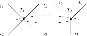
Rule #2: Edge Contractions. At this moment, we can only make up disconnected tensor networks. Edge contractions allow us to link two tensor networks. Suppose we have two ${3}$ dimensional tensor networks. Contracting two edges, one from each, gives us a tensor network of ${4}$ free edges. This now corresponds a tensor of ${4}$ dimensions.

Join two tensor networks by contracting an edge

We name the contracted edge as ${k}$ . The definition of ${T}$ is

$\displaystyle T(i_1,i_2,j_1,j_2) =\sum_k T_1(i_1,i_2, k) T_2(j_1,j_2, k).$

2.2. Useful Examples

Before we move on, let’s take some examples. Keep in mind that the degree of the vertex determines the number of indices (dimensions of this tensor).

note15x — vector inner product ${\langle u,v \rangle}$

vector inner product ${\langle u,v \rangle}$

Here, one needs to remember that an edge between two tensor nodes is a summation over the index corresponding to the edge. For example, in the vector inner product picture, 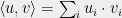${\langle u,v\rangle = \sum_i u_i \cdot v_i}$ , where edge is labeled as ${i}$ . Now you would realize that this picture

is the famous

$\langle u,v \rangle^2 \leq \|u\|^2 \|v\|^2. \quad\quad (\text{Cauchy-Schwarz inequality})$

For us, the most important building block is matrix multiplication. Let ${H=MN}$ . By definition

$H(i,j) = \sum_k M(i,k) N(k, j).$

This is precisely encoded in the picture below.

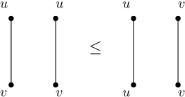
We are ready to talk about matrix product states. In the language of tensor network, a matrix product state is the following picture.

As the degrees indicate, the two boundary vertices ${A_1,A_n}$ represent matrices and the internal vertices represent ${3}$ -dimensional tensors. We can view each matrix as a set of (column) vectors and each ${3}$ -dimensional tensor as a stack of matrices. Then each one of the free edges picks out a vector or a matrix, and the contracted edges multiply them together which gives out a scalar. If this confused you, move on to the next section. I will introduce the formal definition of matrix product states, and you will see that it is just the picture above.

3. Matrix Product States

Before giving the definition, let’s talk about how matrix product state (MPS) naturally arises from the study of quantum states with low entanglement. Matrix product state can be viewed as a generalization of product state—(pure) quantum state with no entanglement. Let’s consider a simple product state ${|\psi\rangle}$ of ${2}$ qubits. It can be factorized:

$\displaystyle |\psi\rangle = \left(\sum_{i=0}^1 \alpha_1^i\ |i\rangle \right)\left(\sum_{j=0}^1 \alpha_2^j \ |j\rangle\right)\nonumber = \sum_{i,j=0}^1 \alpha_1^i \alpha_2^j\ |ij\rangle \ \ \ \ \ (1)$

This state is described by ${4}$ complex scalars ${\left\{\alpha_1^0,\alpha_1^1,\alpha_2^0,\alpha_2^1\right\}}$ , and there is nothing quantum about it. However, if the state has entanglement among its qubits, then we know that it is impossible to be factorized and thereby written as (1). MPS generalizes the form of (1) by replacing the scalars with matrices and vectors.

More formally, a matrix product state starts with the following setup. For an ${n}$ -qudit system, we associate

a qudit in ${\{1,n\}}$ with ${d}$ vectors ${\left\{A_1^{j_1}\right\}, \left\{A_n^{j_n}\right\} \in \mathbb{R}^D}$ ; and
a qudit ${i}$ in ${\{2,3,\cdots, n-1\}}$ with ${d}$ matrices ${\left\{A_i^{j_i}\right\}\in \mathbb{R}^{D\times D}}$ .

Here, ${j_i}$ range from ${0}$ to ${d-1}$ , and ${D}$ is called bond dimension. One can think of the set of vectors as a ${D}$ by ${d}$ matrix and the set of matrices as a ${d}$ by ${D}$ by ${D}$ three-dimensional tensor. Then let them correspond to the vertices in MPS picture. With this setup, a quantum state is in matrix product state if it can be written as

$|\psi\rangle = \sum_{j_1,\cdots,j_n=1}^n A_1^{j_1} A_2^{j_2} \cdots A_n^{j_n} |j_1 j_2\cdots j_n\rangle.$

It is important to keep in mind that ${A_1^{j_1},A_n^{j_n}}$ are two vectors, and the other inner terms are matrices, and we get a scalar from the product. Thus, this represents the tensor ${T(j_1,j_2,\cdots, j_n) = A_1^{j_1} A_2^{j_2} \cdots A_n^{j_n}}$ .

Now back to the picture,

notice that each amplitude ${ A_1^{j_1} A_2^{j_2} \cdots A_n^{j_n}}$ from the equation above is an output of the tensor in the picture, where the free edges take values ${j_1, j_2 ,\cdots, j_n}$ . Also, as discussed earlier, the contracted edges in MPS tensor network correspond to matrix and vector multiplications, so the tensor ${T}$ is precisely represented by the picture.

The complexity of the MPS is closely related to the bond dimension ${D}$ . In particular, the number of parameters in this model is ${O(ndD^2)}$ . We would expect that with higher ${D}$ , we may describe quantum states of more entanglement. In other words, the representation power of an MPS increases with ${D}$ . In principle, one can represent any quantum state as an MPS; however, ${D}$ can be exponentially large. See, e.g., Section 4.1.3 of~\cite{schollwock2011density} for a proof. On the other extreme, the product state example shows that if ${D=1}$ , one can represent and only represent unentangled states. To summarize, here is the picture you should keep in mind.

note33x — Representation power of MPS increases with bond dimension D.

4. Density Matrix Renormalization Group

We are now ready to describe Density Matrix Renormalization Group, proposed originally in [Whi92, Whi93]. As mentioned earlier, it does not come with provable guarantees. In fact, one can construct artificial hard instances such that the algorithm get stuck at certain local minima [SCV08]. However, it has remained one of the most successful heuristics for ${1}$ D systems. We refer the readers to [Sch11] for a complete survey.

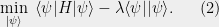
DMRG is a simple alternating minimization scheme for computing the ground state of a ${1}$ D Hamiltonian. We start with an arbitrary MPS. Then each step we optimize over the set of matrices ${\left\{A_i^{j_i}\right\}_{j_i=0}^d}$ associated with site ${i}$ , while fixing everything else, and iterate until convergence. (You may wonder if one can simultaneously optimize over multiple sites. It turns out that it is an NP-hard problem [Eis06].)

Formally, the Hamiltonian problem can be phrased as a eigenvalue problem given a Hermitian matrix ${H}$ , and thus we want to optimize over all ${|\psi\rangle}$ in MPS of a fixed bond dimension ${D}$

$\min_{|\psi\rangle}\frac{\langle \psi| H | \psi \rangle}{\langle \psi ||\psi \rangle}.$

Here, we assume that the input Hamiltonian is in the product form. In particular, it means that it can be written as a tensor network as

note36x — Input ${1}$ D Hamiltonian is of the particular product form.

Input ${1}$ D Hamiltonian is of the particular product form.

so the numerator of the optimization objective looks like

note37x

The DMRG works with the Langrangian of the objective. For some ${\lambda>0}$ , we will consider

$\displaystyle \min_{|\psi\rangle}\,\, {\langle \psi| H | \psi \rangle} - \lambda {\langle \psi ||\psi \rangle}. \ \ \ \ \ (2)$

DMRG optimizes over the set of matrices associated with one qudit. Both terms in (2) are quadratic in this set of matrices.

note39x — The Langrangian ${{\langle \psi| H | \psi \rangle} - \lambda {\langle \psi ||\psi \rangle}}$ as a tensor network.

The Langrangian ${{\langle \psi| H | \psi \rangle} - \lambda {\langle \psi ||\psi \rangle}}$ as a tensor network.

Now to optimize over the set of parameters associated with one site, calculus tells you to set the (partial) derivative to ${0}$ , and the derivative of a quadratic thing is linear. Without going through any algebra, we can guess that the derivative of with respect to a particular site, say the second one, is the same picture except removing the second site on one side.

note40x — The derivative that we set to ${0}$ and solve.

The derivative that we set to ${0}$ and solve.

Notice that the unknown is still there, on the bottom side of each term. The trick of DMRG is to view the rest of the network as a linear map applied to the unknown.

note41x

Given ${H'}$ and ${B}$ , we now have a clean numerical linear algebra problem of solving

$\displaystyle H'x = \lambda Bx. \ \ \ \ \ (3)$

This is called a generalized eigenvalue problem, and it is well studied. Importantly, for ${1}$ D systems, ${H'}$ is typically very sparse, which enables very fast solvers in practice. Finally, DMRG sweeps over the sites one after another and stops until convergence is achieved.

5. Concluding Remarks

Our presentation of tensor networks and MPS roughly follows [GHLS15], a nice introductory survey on quantum Hamiltonian complexity.

The notion of tensor networks extends well beyond 1D systems, and a generalization of MPS is called tensor product state. It leads to algorithms for higher dimensional quantum systems. One may read [CV09] for a comprehensive survey.

Tensor network has been interacting with other concepts. Within physics, it has been used in quantum error correction [FP14, PYHP15], conformal field theory [Orú14], and statistical mechanics [EV15]. In TCS , we have found its connections with Holographic algorithms [Val08, CGW16], arithmetic complexity [BH07, CDM16, AKK19], and spectral algorithms [MW18]. In machine learning, it has been applied to probabilistic graphical models [RS18], tensor decomposition [CLO16], and quantum machine learning [HPM18].

For DMRG, we have only given a rough outline, with many details omitted, such as how to set ${D}$ and ${\lambda}$ and how to obtain the Hamiltonian in the matrix product form, and how to compute the linear maps ${H'}$ and ${B}$ for each iteration. An interested reader may read [Sch05, Sch11].

References

[AKK19] Per Austrin, Peeri Kaski, and Kaie Kubjas. Tensor network complexity of multilinear maps. In Proceedings of the 2019 Conference on Innovations in Theoretical Computer Science. ACM, 2019.

[BH07] Martin Beaudry and Markus Holzer. The complexity of tensor circuit evaluation. Computational Complexity, 16(1):60, 2007.

[CDM16] Florent Capelli, Arnaud Durand, and Stefan Mengel. e arithmetic complexity of tensor contraction. eory of Computing Systems, 58(4):506{527, 2016.

[CGW16] Jin-Yi Cai, Heng Guo, and Tyson Williams. A complete dichotomy rises from the capture of vanishing signatures. SIAM Journal on Computing, 45(5):1671{1728, 2016.

[CLO16] Andrzej Cichocki, Namgil Lee, Ivan V Oseledets, A-H Phan, Qibin Zhao, and D Mandic. Low-rank tensor networks for dimensionality reduction and large-scale optimization problems: Perspectives and challenges part 1. arXiv preprint arXiv:1609.00893, 2016.

[CV09] J Ignacio Cirac and Frank Verstraete. Renormalization and tensor product states in spin chains and laices. Journal of Physics A: Mathematical and Theoretical, 42(50):504004, 2009.

[Eis06] Jens Eisert. Computational difficulty of global variations in the density matrix renormalization group. Phys. Rev. Le., 97:260501, Dec 2006.

[EV15] G. Evenbly and G. Vidal. Tensor network renormalization. Phys. Rev. Le., 115:180405, Oct 2015.

[FP14] Andrew J Ferris and David Poulin. Tensor networks and quantum error correction. Phys. Rev. Le., 113(3):030501, 2014.

[FSW07] Holger Fehske, Ralf Schneider, and Alexander Weie. Computational Many-Particle Physics. Springer, 2007.

[GHLS15] Sevag Gharibian, Yichen Huang, Zeph Landau, and Seung Woo Shin. Quantum Hamiltonian complexity. Foundations and Trends in Theoretical Computer Science, 10(3):159, 2015.

[HPM18] William James Huggins, Piyush Patil, Bradley Mitchell, K Birgia Whaley, and Miles Stoudenmire. Towards quantum machine learning with tensor networks. Quantum Science and Technology, 2018.

[MW18] Ankur Moitra and Alexander S Wein. Spectral methods from tensor networks. arXiv preprint arXiv:1811.00944, 2018.

[Orú14] Román Orús. Advances on tensor network theory: symmetries, fermions, entanglement, and holography. e European Physical Journal B, 87(11):280, 2014.

[PYHP15] Fernando Pastawski, Beni Yoshida, Daniel Harlow, and John Preskill. Holographic quantum error-correcting codes: Toy models for the bulk/boundary correspondence. Journal of High Energy Physics, 2015(6):149, 2015.

[RS18] Elina Robeva and Anna Seigal. Duality of graphical models and tensor networks. Information and Inference: A Journal of the IMA, 2018.

[Sch05] Ulrich Schollwöck. The density-matrix renormalization group. Rev. Mod. Phys., 77(1):259, 2005.

[Sch11] Ulrich Schollwöck. The density-matrix renormalization group in the age of matrix product states. Annals of Physics, 326(1):96, 2011.

[SCV08] Norbert Schuch, Ignacio Cirac, and Frank Verstraete. Computational difficulty of finding matrix product ground states. Phys. Rev. Le., 100(25):250501, 2008.

[Val08] Leslie G Valiant. Holographic algorithms. SIAM Journal on Computing, 37(5):1565, 2008.

[Whi92] Steven R. White. Density matrix formulation for quantum renormalization groups. Phys. Rev. Le., 69:2863, Nov 1992.

[Whi93] Steven R. White. Density-matrix algorithms for quantum renormalization groups. Phys. Rev. B, 48:10345, Oct 1993.

	Mostafa Touny on Avi wins the Turing, TCS for…
	Harvard Professors o… on Open letter to the Harvard…
	Harvard Professors o… on Open letter to the Harvard…
	Harvard, we have a p… on Letter to the Harvard Corporat…
	Eitan bachmat on Letter to the Harvard Corporat…

Tensor Networks, Matrix Product States and Density Matrix Renormalization Group

Published by Fred Zhang

3 thoughts on “Tensor Networks, Matrix Product States and Density Matrix Renormalization Group”

Leave a comment Cancel reply

Share this:

Related

Published by Fred Zhang

3 thoughts on “Tensor Networks, Matrix Product States and Density Matrix Renormalization Group”

Leave a comment Cancel reply