Replica Method for the Machine Learning Theorist: Part 1 of 2

Blake Bordelon, Haozhe Shan, Abdul Canatar, Boaz Barak, Cengiz Pehlevan

[Boaz’s note: Blake and Haozhe were students in the ML theory seminar this spring; in that seminar we touched on the replica method in the lecture on inference and statistical physics but here Blake and Haozhe (with a little help from the rest of us) give a great overview of the method and its relations to ML. See also all seminar posts.]

I. Analysis of Optimization Problems with Statistical Physics

In computer science and machine learning, we are often interested in solving optimization problems of the form

$\min_{x \in \mathcal{S}} H(x,\mathcal D)$

where $H$ is an objective function which depends on our decision variables $x \in \mathcal S$ as well as on a set of problem-specific parameters $\mathcal D$ . Frequently, we encounter problems relevant to machine learning, where $\mathcal D$ is a random variable. The replica method is a useful tool to analyze large problems and their typical behavior over the distribution of $\mathcal D$ .

Here are a few examples of problems that fit this form:

In supervised learning, $H$ may be a training loss, $x$ a set of neural network weights and $\mathcal D$ the data points and their labels
We may want to find the most efficient way to visit all nodes on a graph. In this case $\mathcal D$ describes nodes and edges of the graph, $x$ is a representation of the set of chosen edges, and $H$ can be the cost of $x$ if $x$ encodes a valid path and $\infty$ (or a very large number ) if it doesn’t encode a valid path.
Satisfiability: $x \in \{0,1\}^N$ is a collection booleans which must satisfy a collection of constraints. In this case the logical constraints (clauses) are the parameters $\mathcal D$ . $H(x)$ can be the number of constraints violated by $x$ .
Recovery of structure in noisy data: $x$ is our guess of the structure and $\mathcal D$ are instances of the observed noisy data. For example PCA attempts to identify the directions of maximal variation in the data. With the replica method, we could ask how the accuracy of the estimated top eigenvector degrades with noise.

II. The Goal of the Replica Method

The replica method is a way to calculate the value of some statistic (observable in physics-speak) $O(x)$ of $x$ where $x$ is a “typical” minimizer of $H(x,\mathcal{D})$ and $\mathcal{D}$ is a “typical” value for the parameters (which are also known in physics-speak as the disorder).

In Example 1 (supervised learning), the observable may be the generalization error of a chosen algorithm (e.g. a linear classifier) on a given dataset. For Example 2 (path), this could be the cost of the best path. For Example 3 (satisfiability), the observable might be whether or not a solution exists at all for the problem. In Example 4 (noisy data), the observable might be the quality of decoded data (distance from ground truth under some measure).

An observable like generalization error obviously depends on $\mathcal{D}$ , the problem instance. However, can we say something more general about this type of problem? In particular, if $\mathcal D$ obeys some probability distribution, is it possible to characterize the the typical observable over different problem instances $\mathcal D$ ?

For instance, in Example 1, we can draw all of our training data from a distribution. For each random sample of data points $\mathcal D$ , we find the set of $x$ which minimize $H(x, \mathcal D)$ and compute a generalization error. We then repeat this procedure many times and average the results. Sometimes, there are multiple $x$ that minimize $H$ for a given sample of $\mathcal{D}$ ; this requires averaging the observable over all global minima for each $\mathcal{D}$ first, before averaging over different $\mathcal D$ .

To give away a “spolier”, towards the end of this note, we will see how to use the replica method to give accurate predictions of performance for noisy least square fitting and spiked matrix recovery.

Generalization gap in least squares ridge regression, figure taken from Canatar, Bordelon, and Pehlevan

Performance (agreement with planted signal) as function of signal strength for spiked matrix recovery, as the dimension grows, the experiment has stronger agreement with theory. See also Song Mei’s exposition

A. What do we actually do?

Now that we are motivated, let’s see what quantities the replica method attempts to obtain. In general, given some observable $O(x,\mathcal D)$ , the average of $O$ over a minimizer $x$ chosen at random from the set $\text{arg} \min H(x,\mathcal{D})$ , and take the average of this quantity over the choice of the disorder $\mathcal{D}$ .
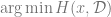
In other words, we want to compute the following quantity:

$\text{Desired quantity } = \mathbb{E}_{\mathcal{D}} \mathbb{E}_{x \in \text{arg}\min H(x,\mathcal{D})} \left[ O(x, \mathcal{D}) \right]$

The above equation has two types of expectation- over the disorder $D$ , and over the minimizers $x$ .
The physics convention is to

use $\left< f \right>_{\mathcal D}$ for the expectation of a function $f(\mathcal{D})$ over the disorder $\mathcal{D}$
use $\int g(x) \mu(x) dx$ for the expectation of a function $g(x)$ over $x$ chosen according to some measure $\mu$ .

Using this notation, we can write the above as

$\text{Desired quantity } = \left< \int p^*(x;\mathcal D) O(x,\mathcal D) dx \right>_{\mathcal D}$

where $\left< \right>_{\mathcal D}$ denotes an average over the probability measure for problem parameters $\mathcal D$ , and $p^*(x;\mathcal D)$ is a uniform distribution over the set of $x$ that minimize $H(x,\mathcal{D})$ with zero probability mass placed on sub-optimal points.

The ultimate goal of the replica method is to express

$\text{Desired quantity } = \text{solution of optimization on constant number of variables}$

but it will take some time to get there.

B. The concept of “self-averaging” and concentration

Above, we glossed over an important distinction between the “typical” value of $f(\mathcal D) = \int p^*(x; \mathcal D) O(x,\mathcal D) dx$ and the *average* value of $f(\mathcal D)$ . This is OK only when we have concentration in the sense that with high probability over the choice of $\mathcal{D}$ , $f(\mathcal{D})$ is close to its expected value. We define this as the property that with probability at least $1-\epsilon$ , the quantity $f(\mathcal{D})$ is within a $1\pm \epsilon$ multiplicative factor of its expectation, whwere $\epsilon$ is some quantity that goes to zero as the system size grows. A quantity $f(\cdot)$ that concentrates in this sense is called self averaging.

For example, suppose that $X= \sum_{i=1}^n X_i$ where each $X_i$ equals $1$ with probabilty $1/2$ and $0$ with probability $1/2$ independently. Standard Chernoff bounds show that with high probability $X \in [n/2 \pm O(\sqrt{n})]$ or $\tfrac{X}{\mathbb{E} X} \in \left(1 + O(\tfrac{1}{\sqrt n})\right)$ . Hence $X$ is a self averaging quantity.

In contrast the random variable $Y=2^X$ is not self averaging. Since $Y = \prod_{i=1}^n 2^{X_i}$ and these random variables are independent, we know that $\mathbb{E} Y = \prod_{i=1}^n \mathbb{E} 2^{X_i} = \left(\tfrac{1}{2} 2^1 + \tfrac{1}{2} 2^0 \right)^n = (3/2)^n$ . However, with high probability a typical value of $Y$ will be of the form $2^{n/2 \pm O(\sqrt{n})} = \sqrt{2}^{n \pm O(\sqrt n)}$ . Since $\sqrt{2} < 3/2$ we see that the typical value of $Y$ is exponentially smaller than the expected value of $Y$ .

The example above is part of a more general pattern. Often even if a variable $Y$ is not self averaging, the variable $X = \log Y$ will be self-averaging. Hence if we are interested in the typical value of $Y$ , the quantity $\exp\left( \mathbb{E} [\log Y] \right)$ is more representative than the quantity $\mathbb{E}[Y]$ .

C. When is using the replica method a good idea?

Suppose that we want to compute a quantity of the form above. When is it a good idea to use the replica method to do so?
Generally, we would want it to satisfy the following conditions:

The learning problem is high dimensional with a large budget of data. The replica method describes a thermodynamic limit where the system size and data budget are taken to infinity with some fixed ratio between the two quantities. Such a limit is obviously never achieved in reality, but in practice sufficiently large learning problems can be accurately modeled by the method.
The loss or the constraints are convenient functions of $x$ and $\mathcal D$ . Typically $H$ will be a low degree polynomial or a sum of local functions (each depending on small number of variables) in $x$ .
Averages over the disorder in $\mathcal D$ are tractable analytically. That is, we can compute marginals of the distribution over $\mathcal D$ .
The statistic that we are interested in is self-averaging.

If the above conditions aren’t met, it is unlikely that this problem will gain much analytical insight from the replica method.

III. The Main Conceptual Steps Behind Replica Calculations

We now describe the conceptual steps that are involved in calculating a quantity using the replica method.
They are also outlined in this figure:

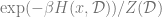
Step 1:”Softening” Constraints with the Gibbs Measure

The uniform measure on minimizers $p^*(x;\mathcal D)$ is often difficult to work with. To aid progress, we can think of it as a special case of what is known as the Gibbs measure, defined as
$p_\beta(x;\mathcal D)dx= \frac{1}{Z(\mathcal D)}\exp \left( -\beta H(x,\mathcal{D})\right)dx$

where $Z(\mathcal D) = \int \exp\left(-\beta {H}(x, \mathcal D) \right)dx$ is the normalization factor, or partition function. $\beta$ is called the inverse temperature, a name from thermodynamics. It is easy to see that when $\beta\to\infty$ (i.e., when the temperature tends to the absolute zero), the Gibbs measure converges to a uniform distribution on the minimizers of $H$ : $p_{\beta} \to p^*$ .

Hence we can write

$\text{Desired quantity } = \left< \int p^*(x;\mathcal D) O(x,\mathcal D) dx \right>{\mathcal D} = \left< \lim_{\beta \rightarrow \infty} \int p_\beta(x;\mathcal D) O(x,\mathcal D) dx \right>_{\mathcal D}$

Physicists often exchange the order of limits and expectations at will, which generally makes sense in this setting, and so assume

$\text{Desired quantity } = \lim_{\beta \rightarrow \infty} \left< \int p_\beta(x;\mathcal D) O(x,\mathcal D) dx \right>_{\mathcal D}$

Thus general approach taken in the replica method is to derive an expression for the average observable for any $\beta$ and then take the $\beta \rightarrow \infty$ limit. The quantity $\int p_\beta(x;\mathcal D) O(x,\mathcal D) dx$ is also known as the thermal average of $O$ , since it is taken with respect to the Gibbs distribution at some positive temperature.

To compute the thermal average of $O$ , we define the following augmented partition function:

$Z(\mathcal D, J) = \int_{S} \exp\left( -\beta H(x,\mathcal D) + J O(x; \mathcal D) \right) dx.$

One can then check that

$\frac{d}{dJ} \log Z(\mathcal{D}, J)\Big|_{J=0}= \frac{1}{Z} \int O(x,\mathcal D) \exp(- \beta H(x,\mathcal D) ) dx = \int p\beta(x;\mathcal D) O(x,\mathcal D) dx$

Hence our desired quantity can be obtained as

$\text{Desired quantity } = \lim_{\beta \to \infty} \frac{\partial}{\partial J} \left< \log Z(\mathcal D, J) \right>_{\mathcal D}(0)$

or (assuming we can again exchange limits at will):

$\text{Desired quantity } = \lim_{\epsilon \to 0} \tfrac{1}{\epsilon}\left[ \lim_{\beta \to \infty} \left< \log Z(\mathcal D, \epsilon) \right>{\mathcal D} - \lim_{\beta \to \infty} \left< \log Z(\mathcal D, 0) \right>_{\mathcal D}\right]$

We see that ultimately computing the desired quantity reduces to computing quantities of the form

$\left< \log Z'(\mathcal{D}) \right>_{\mathcal D}\;\; (\star)$

for the original or modified partition function $Z'$ . Hence our focus from now on will be on computing ( $\star$ ).
Averaging over $\mathcal D$ is known as “configurational average” or quenched average. All together, we obtain the observable, first thermal averaged to get $O^*(\mathcal D)$ (averaged over $p^*(x;\mathcal D)$ ) and then quenched averaged over $\mathcal D$ .

⚠ What Concentrates?: It is not just an algebraic convenience to average $\log Z$ instead of averaging $Z$ itself. When the system size $N$ is large, $\frac{1}{N} \log Z$ concentrates around its average. Thus, the typical behavior of the system can be understood by studying the quenched average $\frac{1}{N} \left< \log Z \right>$ The partition function $Z$ itself often does not concentrate and in general the values $\frac{1}{N} \log \left< Z \right>$ (known as the “annealed average”) and $\frac{1}{N}\left< \log Z \right>$ (known as the “quenched average”) could differ subtantially. For more information, please consult Mezard and Montanari’s excellent book, Chapter 5.

Step 2: The Replica Trick

Hereafter, we use $\langle \cdot \rangle$ to denote the average and drop the dependence of $\mathcal D$ and $J$ . To compute $\left< \log Z(\mathcal D, J) \right>{\mathcal D}$ , we use an identity $\left< \log Z \right> = \lim_{n \to 0} \frac{1}{n} \log \left< Z^n \right>.$

For the limit to make sense, $n$ should be any real number. However, the expression for $Z^n$ is only easily computable for natural numbers. ⚠ This step is non-rigorous: we will obtain an expression for $\log \langle Z^n \rangle$ for natural number $n$ , and then take the $n \rightarrow 0$ limit after the fact.

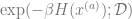
Recall that under the Gibbs distribution $p_\beta(\mathcal D)$ , the probability density on state $x$ is equal to $\exp(-\beta H(x,\mathcal D) )/Z(\mathcal D)$ . Denote by $p_\beta(\mathcal D)^n$ the probability distribution over a tuple $\vec{x} = (x^{(1)},\ldots,x^{(n)})$ of $n$ independent samples (also known as replicas) chosen from $p_\beta(\mathcal D)$ .

Since the partition function $Z$ is an integral (or sum in the discrete case) of the form $\int \exp(-\beta H(x;\mathcal D)) dx$ , we can write $Z(\mathcal D)^n$ as the integral of $\prod_{a=1}^n \exp(-\beta H(x^{(a)};\mathcal D))= \exp\left( - \beta \sum_{a=1}^n H(x^{(a)}, \mathcal D)\right)$ where $x^{(1)},\ldots,x^{(n)}$ are independent variables.

Now since each $x^{(a)}$ is weighed with a factor of $\exp(-\beta H(x^{(a)});\mathcal D)$ , this expression can be shown as equal to taking expectation of some exponential function $\exp( \sum_{a=1}^n G(x^{(a)}; \mathcal D))$ over a tuple $(x^{(1)},\ldots,x^{(n)})$ of $n$ independent samples of replicas all coming from the same Gibbs distribution $p_\beta(\mathcal D)$ corresponding to the same instance $\mathcal D$ .
(The discussion on $G$ is just for intuition – we will not care about the particular form of this $G$ , since soon average it over $\mathcal D$ .)

Hence

$\left< Z^n \right> = \left< \int_{\vec{x} \sim p_*(\mathcal D)^n} \exp\left( - \sum_{a=1}^n G(x^{(a)}, \mathcal D) dx \right) \right>_{\mathcal D}.$

Step 3: The Order Parameters

The above expression is an expectation of an integral, and so we can switch the order of summation, and write it also as

$\left< Z^n \right> = \int_{\vec{x} \sim p_*(\mathcal D)^n} \left< \exp\left( - \sum_{a=1}^n G(x^{(a)}, \mathcal D) \right) \right>_{\mathcal D} dx.$

It turns out that for natural energy functions (for example when $H$ is quadratic in $x$ such as when it corresponds to Mean Squared Error loss), for any tuple of $x^{(1)},\ldots,x^{(n)}$ , the expectation over $\mathcal D$ of $\exp\left( - \beta \sum_{a=1}^n H(x^{(a)}, \mathcal D) \right)$ only depends on the angles between the $x^(a)$ ‘s.
That is, rather than depending on all of these $N$ -dimensional vectors, it only depends on the $n^2$ coefficients $Q_{ab} =\frac{1}{N} x^{(a)}\cdot x^{(b)}$ . The $n\times n$ matrix Q is known as the overlap matrix or order parameters and one can often find a nice analytical function $\mathcal{F}$ whose values are bounded (independently of $N$ ) such that

$\left< \exp\left( - \sum_{a=1}^n G(x^{(a)}, \mathcal D) \right) \right>_{\mathcal D} = \exp(-nN \mathcal{F}(Q))$ .

Hence we can replace the integral over $x^{(1)},\ldots,x^{(n)}$ with an integral over $Q$ and write

$\left< Z^n \right> = \int dQ \exp\left(- n N \mathcal F(Q) \right)$

where the measure $dQ$ is the one induced by the overlap distribution of a tuple $\vec{x} \sim p_\beta(\mathcal D)$ taken for a random choice of the parameters $\mathcal D$ .

Since $Q$ only ranges over a small ( $n^2$ dimensional set), at the large $N$ limit, the integral is dominated by the maximum of its integrand (“method of steepest descent” / “saddle point method”). Let $Q^*$ be the global minimum of $\mathcal F$ (within some space of matrices). We have

$\lim_{N \rightarrow \infty}\left< Z^n \right> = \exp(-n N \mathcal F(Q^* )).$

Once we arrive at this expression, the configurational average of $-\log Z$ is simply $N \mathcal F(Q^*)$ . These steps constitute the replica method. The ability to compute the configurational average by creating an appropriate $Q$ is one of the factors determining whether the replica method can be used. For example, in the supervised learning example, $H$ is almost always assumed to be quadratic in $x$ ; cross-entropy loss, for instance, is generally not amendable.

⚠ Bad Math Warning: there are three limits, $\beta \rightarrow \infty$ , $N \rightarrow \infty$ , and $n \rightarrow 0$ . In replica calculations, we assume that we take take these limits in whichever order that is arithmetically convenient.

Coming up: In part two of this blog post, we will explain the replica symmetric assumption (or “Ansatz” in Physics-speak) on the order parameters $Q$ and then demonstrate how to use the replica method for two simple examples: least squares regression and spiked matrix model.

2 thoughts on “Replica Method for the Machine Learning Theorist: Part 1 of 2”

Pingback: Replica Method for the Machine Learning Theorist: Part 2 of 2 – Windows On Theory
James says:

August 26, 2022 at 4:06 pm

Thank you for the amazing post. Unfortunately, I’m lost at Step:2, specifically in the paragraph where you introduce G. What do you mean each x^{(a)} is weighted with the factor of \exp(-\beta H)?

	Mostafa Touny on Avi wins the Turing, TCS for…
	Harvard Professors o… on Open letter to the Harvard…
	Harvard Professors o… on Open letter to the Harvard…
	Harvard, we have a p… on Letter to the Harvard Corporat…
	Eitan bachmat on Letter to the Harvard Corporat…

Replica Method for the Machine Learning Theorist: Part 1 of 2

Blake Bordelon, Haozhe Shan, Abdul Canatar, Boaz Barak, Cengiz Pehlevan

I. Analysis of Optimization Problems with Statistical Physics