Yet another backpropagation tutorial

(Updated and expanded 12/17/2021)

I am teaching deep learning this week in Harvard’s CS 182 (Artificial Intelligence) course. As I’m preparing the back-propagation lecture, Preetum Nakkiran told me about Andrej Karpathy’s awesome micrograd package which implements automatic differentiation for scalar variables in very few lines of code.

I couldn’t resist using this to show how simple back-propagation and stochastic gradient descents are. To make sure we leave nothing “under the hood” we will not import anything from the package but rather only copy paste the few things we need. I hope that the text below is generally accessible to anyone familiar with partial derivatives. See this colab notebook for all the code in this tutorial. In particular, aside from libraries for plotting and copy pasting a few dozen lines from Karpathy, this code uses absolutely no libraries (no numpy, no pytorch, etc..) and can train (slowly..) neural networks using stochastic gradient descent. (This notebook builds the code more incrementally.)

Automatic differentiation is a mechanism that allows you to write a Python functions such as

def f(x,y): return (x+y)+x**3

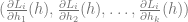
and enables one to automatically obtain the partial derivatives and . Numerically we could do this by choosing some small value and computing both and .
However, if we generalize this approach to variables, we get an algorithm that requires roughly evaluations of . Back-propagation enables computing all of the partial derivatives at only constant overhead over the cost of a single evaluation of .

Backpropagation and the chain rule

Back-propagation is a direct implication of the multi-variate chain rule. Let’s illustrate this for the case of two variables. Suppose that and are differentiable functions, and define

.

That is, we have the following situation:

where is the value

Then the chain rule states that

You can take this on faith, but it also has a simple proof. To see the intuition, note that for small , and . For small , . Hence, if we ignore terms with powers of delta two or higher,

Meaning that which is what we needed to show.

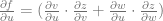
The chain rule generalizes naturally to the case that is a function of more variables than and . Generally, if the value is obtained by first computing some intermediate values from and then computing in some arbitrary way from , then . It also generalizes easily to the case that is not a scalar but a vector of variables.

As a corollary, if you already managed to compute the values , and you kept track of the way that were obtained from , then you can compute .

This suggests a simple recursive algorithm by which you compute the derivative of the final value with respect to an intermediate value in the computation using recursive calls to compute the values for all the values that were directly computed from . Back propagation is this algorithm.

Automatic differentiation via backpropagation

As I describe in my introduction to theoretical computer science text, one can informally define an algorithm as a set of instructions for computing an output from an input by following a sequence of elementary steps. For example, Muhammad ibn Musa al-Khwarizmi (the 9th century Persian scholar on whose name the word “Algorithm” is based) described the algorithm to solve quadratic equations of the form as a sequence of steps.

If were were to translate it into Python, al-Khwarizmi’s equation solving procedure is the following:

from math import sqrt

def solve_eq(b,c):
    # return solution of x^2 + bx = c following Al Khwarizmi's instructions
    # Al Kwarizmi demonstrates this for the case b=10 and c= 39

    val1 = b / 2.0 # "halve the number of the roots"
    val2 = val1 * val1 # "this you multiply by itself"
    val3 = val2 + c # "Add this to thirty-nine"
    val4 = sqrt(val3) # "take the root of this"
    val5 = val4 - val1 # "subtract from it half the number of roots"
    return val5  # "This is the root of the square which you sought for"

The point is that computation of the output from the input is obtained by repeatedly doing the following: compute intermediate values by applying a simple operation to the inputs or previously computed values. The computation graph is the directed acyclic graph with a directed edge from a value u and a value v if u was used in computing v.

The backpropagation algorithm is as follows:

Step 1: Forward Pass

Using the code of , and some assignment for its input, compute by following a sequence of elementary operations applied to intermediate values. While doing this computation, keep track for every intermediate value of both (1) the value of and (2) the way was computed as an elementary function of its immediate predecessors (which we call its “children”).

Step 2: Backward pass

If we let be the output, we now recursively compute for every intermediate value . For the output itself .

Suppose that we have already recursively computed the partial derivative of some intermediate value . And suppose that for some elementary function . where . are ‘s children.

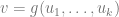
We know the values of from the forward pass. And so we can compute for every child of the contribution of to by computing at the values .

For example, if the function is obtained by computing , and then , then we compute the partial derivatives on the assignment by first making a forward pass (green in the figure below) to compute all the intermediate values and the dependency, and then making a backward pass (brown in the figure below) to compute the partial derivatives of the output with respect to the intermediate values, starting from the output and going to the inputs.

Is Backpropagation “the same as” the chain rule?

The backpropagation algorithm is obtained by repeated applications of the chain rule, and so superficially it might seem that this is the same algorithm for computing derivatives you have learned in your high school or college calculus class. However, it is not the same, a point made by this blog post of Lunjia Hu and also here. The main point is the following.

The approach we have learned in school is to write down the computation as a formula and then first compute the derivative of the output as a function of its immediate children, then compute the derivative of these predecessors as a function of their children and so on and so forth. This approach scales with the formula size for . If we are using intermediate values in the computation more than once, the formula size might be dramatically larger than the circuit size. The key issue with backpropagation is that it only scales with the circuit size, and so it enables computing the gradient as efficiently as computing itself. (Indeed, in 1983 Baur and Strassen independently discovered backpropagation as a way of proving that the circuit complexity of is at most three times the circuit complexity of .)

The efficiency gains of backpropagation are particularly dramatic for neural networks where we (1) are typically only interested in the derivative with respect to a single output (the loss) or just few numbers, (2) neurons of intermediate layers are used by many downstream neurons, and so the circuit size is dramatically smaller than the formula size, and (3) the number of inputs is quite large and so we can’t afford this factor (which will be the case if we use numerical differentiation or forward propagation).

Implementing automatic differentiation using back propagation in Python

We now describe how to do this in Python, following Karpathy’s code. The basic class we use is Value. Every member of Value is a container that holds:

1. The actual scalar (i.e., floating point) value that holds. We call this data.
2. The gradient of with respect to some future unknown value that will use it. We call this grad and it is initialized to zero.
3. Pointers to all the values that were used in the computation of . We call this _prev
4. The method that adds (using the current value of and other values) the contribution of to the gradient of all its previous values to their gradients. We call this function _backward. Specifically, at the time we call _backward we assume that u.grad already contains where is the final value we are interested in. For every value that was used to compute , we add to v.grad the quantity . For the latter quantity we need to keep track of how was computed from .
5. If we call the method backwards (without an underscore) on a variable then this will compute the derivative of with respect to for all values that were used in the computation of (not just the immediate children of ). We do this by applying _backward to and then recursively going over the “children” (values used to compute ) and children’s children etc., calling _backward on each one and keeping track of the ones we visited (just like in the Depth First Search (DFS) algorithm).

Let’s now describe this in code. We start off with a simple version that only supports addition and multiplication. The constructor for the class is the following:

class Value:
    """ stores a single scalar value v 
         and placeholder for derivative d output/ d v"""

    def __init__(self, data, _children=()):
        self.data = data
        self.grad = 0
        self._backward = lambda: None
        self._prev = set(_children)

which fairly directly matches the description above. This constructor creates a value without using prior values, which is why the _backward function is empty.
However, we can also create values by adding or multiplying previously computing ones, by adding the following methods:

  def __add__(self, other):
        other = other if isinstance(other, Value) else Value(other)
        out = Value(self.data + other.data, (self, other))

        def _backward():
            self.grad += out.grad
            other.grad += out.grad
        out._backward = _backward

        return out

    def __mul__(self, other):
        other = other if isinstance(other, Value) else Value(other)
        out = Value(self.data * other.data, (self, other))

        def _backward():
            self.grad += other.data * out.grad
            other.grad += self.data * out.grad
        out._backward = _backward

        return out

We can add or multiply a Value object with either another Value object, or a scalar (int or float). In the latter case, we first convert the scalar into a Value object. If we apply an operation op (e.g. addition or multiplication) to two Value objects self and other then the result is a Value object out such that (1) out.data contains op applied to self.data and other.data and (2) out._backward contains the code that will (after out.grad is computed) propagate backward to self.grad and out.grad the contributions of out to the partial derivatives of the final output with respect to self and other.

For example, if we create by adding the values and , then the _backward function of works by adding w.grad (which equals , where is the final output) to both u.grad and v.grad.

If is obtained by multiplying and then we add w.grad * v.data (in other words ) to u.grad and similarly add w.grad * u.data () to v.grad.

Note that if w is computed as a function of u and v, then to compute the contribution of w to u.grad and w.grad we need to know (1) the partial derivative which is stored at w.grad and (2) the values of u and v which are stored in u.data and v.data.

The backward function is obtained by setting the gradient of the current value to and then running _backwards on all other values in reverse topological order:

def backward(self, visited= None): # slightly shorter code to fit in the blog 
    if visited is None:
        visited= set([self])
        self.grad = 1
    self._backward()
    for child in self._prev:
        if not child in visited:
            visited.add(child)
            child.backward(visited)

For example, if we run the following code

a = Value(5)
def f(x): return (x+2)**2 + x**3
y = f(a)
y.backward()
print(y.data, a.grad)

then the values printed will be 174 and 89 since 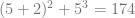the derivative of equals .

In the notebook you can see that we implement also the power function, and have some “convenience methods” (division etc..).

Linear regression using back propagation and stochastic gradient descent

In stochastic gradient descent we are given some data and want to find an hypothesis that minimizes the empirical loss where is a loss function mapping two labels to a real number. If we let be the -th term of this sum, then, identifying with the parameters (i.e., real numbers) that specify it, stochastic gradient descent is the following algorithm:

1. Set to be a random vector. Set to be some small number (e.g., )
2. For (where is the number of epochs):

• For : (in random order)
  • Let

If is specified by the parameters is the vector . This is exactly the vector we can obtain using back propagation.

For example, if we want a linear model, we can use as our parameters and the function will be . We can generate random points X,Y as follows:

Now we can define a linear model as follows:

class Linear:
  def __init__(self):
    self.a,self.b = Value(random.random()),Value(random.random())
  def __call__(self,x): return self.a*x+self.b

  def zero_grad(self):
    self.a.grad, self.b.grad = 0,0

And train it directly by using SGD:

η = 0.03, epochs = 20
for t in range(epochs):
  for x,y in zip(X,Y):
    model.zero_grad()
    loss = (model(x)-y)**2
    loss.backward()
    model.a , model.b = (model.a - η*model.a.grad  , model.b - η*model.b.grad)

Which as you can see works very well:

From linear classifiers to Neural Networks.

The above was somewhat of an “overkill” for linear models, but the beauty of automatic differentiation is that we can easily use more complex computation.

We can follow Karpathy’s demo and us the same approach to train a neural network.

We will use a neural network that takes two inputs and has two hidden layers of width 16. A neuron that takes input will apply the ReLU function () to where are its weight parameters. (It’s easy to add support for relu for our Value class, see the colab notebook. Also we won’t have a bias term in this example.)

The code for this Neural Network is as follows: (when Value() is called without a parameter the value is random number in )

def neuron(weights,inputs, relu =True):
  # Evaluate neuron with given weights on given inputs
  v =  sum(weights[i]*x for i,x in enumerate(inputs))
  return v.relu() if relu else v


class Net:
  # Depth 3 fully connected neural net with one two inputs and output
  def __init__(self,  N=16):
    self.layer_1 = [[Value(),Value()] for i in range(N)]
    self.layer_2 = [ [Value() for j in range(N)] for i in range(N)]
    self.output =  [ Value() for i in range(N)]
    self.parameters = [v for L in [self.layer_1,self.layer_2,[self.output]] for w in L for v in w]


  def __call__(self,x):
    layer_1_vals = [neuron(w,x) for w in self.layer_1]
    layer_2_vals = [neuron(w,layer_1_vals) for w in self.layer_2]
    return neuron(self.output,layer_2_vals,relu=False) 
    # the last output does not have the ReLU on top

  def zero_grad(self):
    for p in self.parameters:
      p.grad=0

We can train it in the same way as above.
We will follow Karpathy and train it to classify the following points:

The training code is very similar, with the following differences:

• Instead of the square loss, we use the function which is if . This makes sense since our data labels will be and we say we classify correctly if we get the same sign. We get zero loss if we classify correctly all samples with a margin of at least .
• Instead of stochastic gradient descent we will do standard gradient descent, using all the datapoints before taking a gradient step. The optimal for neural networks is actually often something in the middle – batch gradient descent where we take a batch of samples and perform the gradient over them.

The resulting code is the following:

for t in range(epochs):
  loss = sum([(1+ -y*model(x)).relu() for (x,y) in zip(X,Y)])/len(X)
  model.zero_grad()
  loss.backward()
  for p in model.parameters:
    p.data -= η*p.grad

If we use this, we get a decent approximation for this training set (see image below). As Karpathy shows, by adjusting the learning rate and using regularization, one can in fact get 100% accuracy.

Here is an animation demonstrating how training evolves for (a variant of) this net on a different dataset:

Update 11/30: Thanks to Gollamudi Tarakaram for pointing out a typo in a previous version. Update 12/17/21: Significantly extended, inspired by post of Lunjia Hu.