Full-replica-symmetry-breaking based algorithms for dummies

One of the fascinating lines of research in recent years has been a convergence between the statistical physics and theoretical computer science points of view on optimization problems.
`
This blog post is mainly a note to myself (i.e., I’m the “dummy” 😃), trying to work out some basic facts in some of this line of work. it was inspired by this excellent talk of Eliran Subag, itself part of a great Simons institute workshop which I am still planning to watch the talks of. I am posting this in case it’s useful for others, but this is quite rough, missing many references, and I imagine I have both math mistakes as well as inaccuracies in how I refer to the literature – would be grateful for comments!

Screen shot from Eliran Subag’s talk demonstrating the difference between “easy” and “hard” instances.

In computer science, optimization is the task of finding an assignment $x_1,\ldots,x_n$ that minimizes some function $J(x_1,\ldots,x_n)$ . In statistical physics we think of $x_1,\ldots,x_n$ as the states of $n$ particles, and $J(x_1,\ldots,x_n)$ as the energy of this state. Finding the minimum assignment corresponds to finding the ground state, and another computational problem is sampling from the Gibbs distribution where the probability of $x$ is proportional to $\exp(-\beta J(x))$ for some $\beta>0$ .

Two prototypical examples of such problems are:

Random 3SAT – in this case $x\in { \pm 1 }^n$ and $J(x)$ is the number of clauses violated by the assignment $x$ for a random formula.
Sherrington-Kirpatrick model – in this case $x \in { \pm 1 }^n$ and $J(x)= \sum_{i,j} J_{i,j}x_ix_j$ where $J_{i,j}$ are independent normal variables with variance $1/n$ for $i\neq j$ and variance $2/n$ for $i=j$ . (Another way to say it is that $J$ is the matrix $A+A^\top$ where $A$ ‘s entries are chosen i.i.d from $N(0,\tfrac{1}{2n}))$ .)

The physics and CS intuition is that these two problems have very different computational properties. For random 3SAT (of the appropriate density), it is believed that the set of solutions is “shattered” in the sense that it is partitioned to exponentially many clusters, separated from one another by large distance. It is conjectured that in this setting the problem will be computationally hard. Similarly from the statistical physics point of view, it is conjectured that if we were to start with the uniform distribution (i.e., a “hot” system) and “lower the temperature” (increase $\beta$ ) at a rate that is not exponentially slow then we will get “stuck” at a “metastable” state. This is analogous how when we heat up sand and then cool it quickly then rather than returning to its original state, the sand will get stuck at the metastable state of glass.

In contrast for the Sherrington-Kirpatrick (SK) model, the geometry is more subtle, but interestingly this enables better algorithms. The SK model is extermely widely studied, with hundreds of papers, and was the inspiration for the simulated annealing algorithm. If memory serves me right, Sherrington and Kirpatrick made the wrong conjecture on the energy of the ground state, and then Parisi came up in 1979 with a wonderful and hugely influential way to compute this value. Parisi’s calculation was heuristic, but about 30 years later, first Talagrand and later Panchenko proved rigorously many of Parisi’s conjectures. (See this survey of Panchenko.)

Recently Montanari gave a polynomial time algorithm to find a state with energy that is arbitrarily close to the ground state’s. The algorithm relies on Parisi’s framework and in particular on the fact that the solution space has a property known as “full replica symmetry breaking (RSB)” / “ultrametricity”. Parisi’s derivations (and hence also Montanari’s analysis) are highly elaborate and I admit that I have not yet been able to fully follow it. The nice thing is that (as we’ll see) it is possible to describe at least some of the algorithmic results without going into this theory. In the end of the post I will discuss a bit some of the relation to this theory, which is the underlying inspiration for Subag’s results described here.

Note: These papers and this blog post deal with the search problem of finding a solution that minimizes the objective. The refutation problem of certifying that this minimum is at least $-C$ for some $C$ has often been studied. The computational complexity of these problems need not be identical. In particular there are cases where the search problem has an efficient algorithm achieving value $-C^*$ but the best refutation algorithm can only certify that the value is at most $-C'$ for $C' \gg C^*$ .

Analysis of a simpler setting

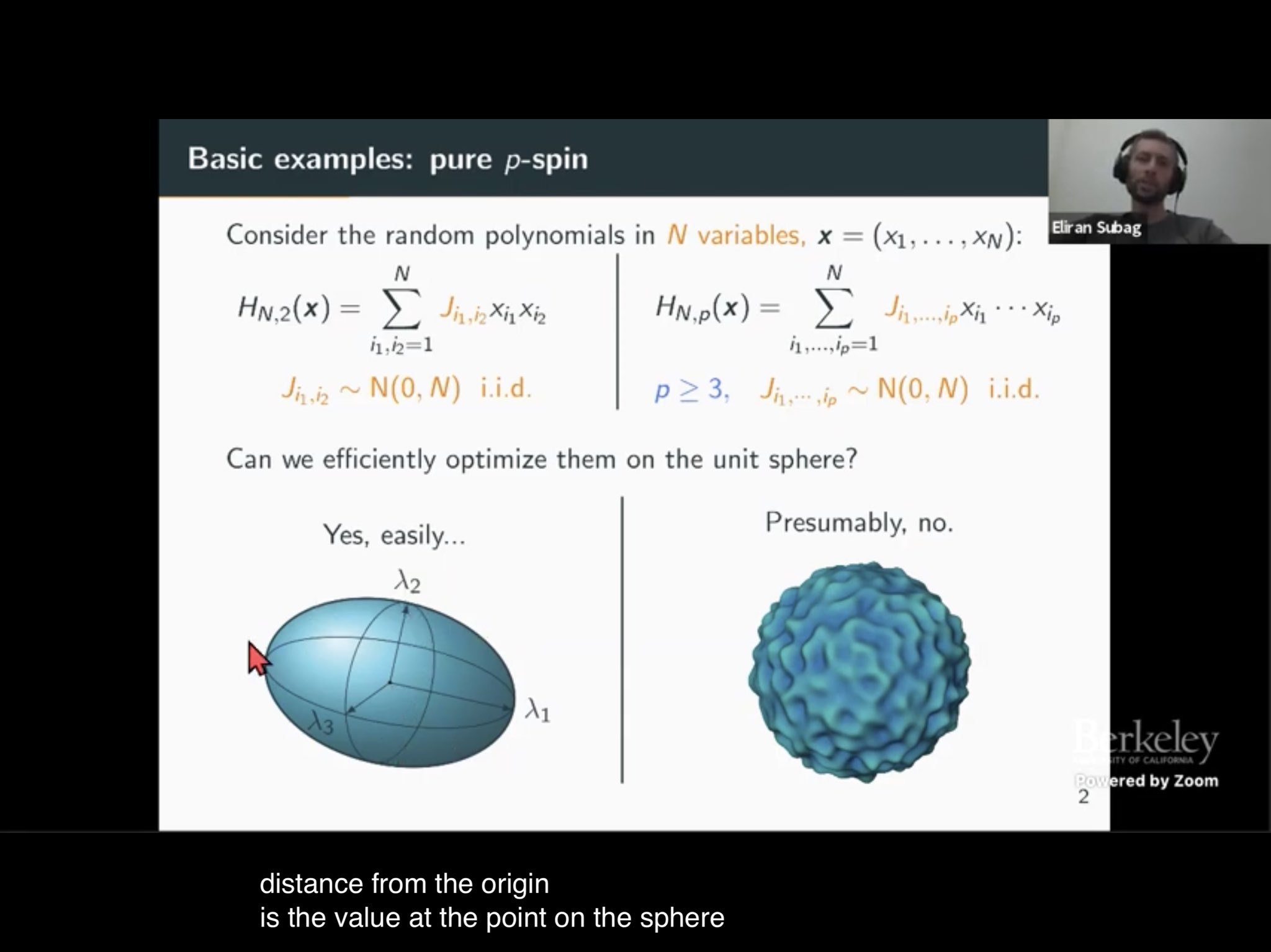
Luckily, there is a similar computational problem, for which the analysis of analogous algorithm, which was discovered by Subag and was the partial inspiration for Montanari’s work, is much simpler. Specifically, we consider the case where $x$ is an element of the unit sphere, and $J(x)$ is a degree $d$ polynomial with random Gaussian coefficients. Specifically, for every vector $\gamma = (\gamma_2,\ldots,\gamma_d)$ , we let $J(x) = \gamma_2 J^2 \cdot x^{\otimes 2} + \gamma_3 J^3 \cdot x^{\otimes 3} + \cdots + \gamma_d J^d \cdot x^{\otimes p}$ where for every $p \in {2,\ldots, d }$ , $J_p$ is a random tensor of order $p$ whose $n^p$ coefficients are all chosen i.i.d in $N(0,1/n)$ . (We assume that polynomial does not have constant or linear components.)

Depending on $\gamma$ , the computational and geometrical properties of this problem can vary considerably. The case that $\gamma = (1,0,\ldots,0)$ (i.e., only $J^2$ has a non-zero coeffiecent) corresponds to finding the unit vector $x$ minimizing $x^\top J x$ for a random matrix $x$ , which of course corresponds to the efficiently solveable minimum eigenvector problem. In contrast, the case $\gamma = (0,1,0,\ldots,0)$ corresponds to finding a rank one component of a random three-tensor, which is believed to be computationally difficult. The Parisi calculations give a precise condition $P$ on the vector $\gamma$ such that if $P(\gamma)$ holds then the solution space has the “full RSB” property (and hence the problem is computationally easy) and if $P(\gamma)$ does not hold then the solution space does not have this property (and potentially the problem is hard).

These calculations also give rise to the following theorem:

Theorem (Chen and Sen, Proposition 2): If $P(\gamma)$ holds then in the limit $n \rightarrow \infty$ , $\min_{x : |x|=1} J(x) = -\int_0^1 \sqrt{\nu''(q)} dq$ , where $\nu(q) = \sum_{p \geq 2} \gamma_p^2 q^p$ . (That is, $\nu''$ is the second derivative of this univariate polynomial)

We will not discuss the proof of this theorem, but rather how, taking it as a black box, it leads to an algorithm for minimizing $J(x)$ that achieves a near-optimal value (assuming $P(\gamma)$ holds).

It is a nice exercise to show that for every two vectors $x,x'\in\mathbb{R}^n$ , $\mathbb{E}_J [J(x)J(x')] = \nu(\langle x,x' \rangle)/n$ . Hence for any unit vector $x$ , $J(x)$ is a random variable with mean zero and standard deviation $\sqrt{\nu(1)/n}$ . Since (after some coarsening) the number of unit vectors of dimension $n$ can be thought of as $c^n$ for some $c>1$ , and we expect the probability of deviating $t$ standard deviations to be $\exp(-c' t^2)$ , the minimum value of $J(x)$ should be $-c'' \sqrt{\nu(1)}$ for some constant $c''$ . However determining this constant is non trivial and is the result of the Parisi theory.

To get a better sense for the quantity $-\int_0^1 \sqrt{\nu''(q)} dq$ , let’s consider two simple cases:

If $\gamma = (1,0,\ldots)$ (i.e., $J(x) = \sum_{i,j}M_{i,j}x_ix_j$ for random matrix $M$ ) then $\nu(q)= q^2$ and $\nu''(q) = 2$ , meaning that $-\int_0^1 \sqrt{\nu''(q)} dq = -\sqrt{2}$ . This turns out to be the actual minimum value. Indeed in this case $\min_{|x|^2=1} J(x) = \tfrac{1}{2} \lambda_{min}(M + M^\top)$ . But the matrix $A=\tfrac{1}{2}(M+M^\top)$ ‘s non diagonal entries are distributed like $N(0,\tfrac{1}{2n})$ and the diagonal entries like $N(0,\tfrac{1}{n})$ which means that $A$ is distributed as $\tfrac{1}{\sqrt{2}}$ times a random matrix $B$ from the Gaussian Orthogonal Ensemble (GOE) where $B_{i,j} \sim N(0,1/n)$ for off diagonal entries and $B_{i,i} \sim N(0,2/n)$ for diagonal entries. The minimum eigenvalue of such matrices is known to be $-2\pm o(1)$ with high probability.
If $\gamma = (0,\ldots,1)$ (i.e. $J(x) = T \cdot x^{\otimes d}$ for a random $d$ -tensor $T$ ) then $P(\gamma)$ does not hold. Indeed, in this case the value $-\int_0^1 \sqrt{\nu''(q)} dq = - \int_0^1 \sqrt{d (d-1)q^{d-2}} dq = - \sqrt{d(d-1)}\tfrac{1}{d/2-1} \approx -2$ for large $d$ . However I believe (though didn’t find the reference) that the actual minimum tends to $-\infty$ with $d$ .

While the particular form of the property $P(\gamma)$ is not important for this post, there are several equivalent ways to state it, see Proposition 1 in Subag’s paper. One of them is that the function $\nu''(t)^{-1/2}$ (note the negative exponent) is concave on the interval $(0,1]$ .
It can be shown that this condition cannot be satisfied if $\gamma_2 = 0$ , and that for every setting of $\gamma_3,\ldots,\gamma_d$ , if $\gamma_2$ is large enough then it will be satisfied.

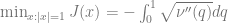
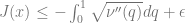
The central result of Subag’s paper is the following:

Theorem: For every $\epsilon>0$ , there is a polynomial-time algorithm $A$ such that on input random $J$ chosen according to the distribution above, with high probability $A(J)=x$ such that $J(x) \leq -\int_0^1 \sqrt{\nu''(q)} dq + \epsilon$ .

The algorithm itself, and the idea behind the analysis are quite simple. In some sense it’s the second algorithm you would think of (or at least the second algorithm according to some ordering).

The first algorithm one would think of is gradient descent. We start at some initial point $x^0$ , and repeat the transformation $x^{t+1} \leftarrow x^t - \eta \nabla J(x^t)$ for some small $\eta$ (and normalizing the norm). Unfortunately, we will generally run into saddle points when we do so, with the gradient being zero. In fact, for simplicity, below we will always make the pessimistic assumption that we are constantly on a saddle point. (This assumption turns out to be true in the actual algorithm, and if it was not then we can always use gradient descent until we hit a saddle.)

The second algorithm one could think of would be to use the Hessian instead of the gradient. That is, repeat the transformation $x^{t+1} \leftarrow x^t - \eta u$ where $u$ is the minimal eigenvector of $\nabla^2 J(x^t)$ (i.e., the Hessian matrix $H$ such that $H_{i,j} = \tfrac{\partial J(x^t)}{\partial x_i \partial x_j}$ ). By the Taylor approximation $J(x - \eta u) \approx J(x) - \eta \nabla J(x) \cdot u + \tfrac{1}{2} \eta^2 u^\top \nabla^2 J(x) u$ (and since we assume the gradient is zero) the change in the objective will be roughly $\tfrac{1}{2} \eta^2 \lambda_{min}(\nabla^2 J(x^t))$ . (Because we assume the gradient vanishes, it will not make a difference whether we update with $-\eta u$ or $+\eta u$ , but we use $-\eta$ for consistency with gradient descent.)

The above approach is promising, but we still need some control over the norm. The way that Subag handles this is that he starts with $x^0 = 0$ , and at each step takes a step in an orthogonal direction, and so within $1/\eta^2$ steps he will get to a unit norm vector. That is, the algorithm is as follows:

Algorithm:

Input: $J:\mathbb{R}^n \rightarrow \mathbb{R}$ .

Goal: Find unit $x$ approximately minimizing $J(x)$

Initialize $x^0 = 0^n$
For $t=0,\ldots,1/\eta^2-1$ : i. Let $u^t$ be a unit vector $u$ such that $u$ is orthogonal to $u^0,\ldots,u^{t-1}$ and $u^\top \nabla^2 J(x^t) u \approx \lambda_{min}(\nabla^2 J(x^t))$ . (Since the bottom eigenspace of $\nabla^2 J(x^t)$ has large dimention, we can find a vector $u$ that is not only nearly minimal eigenvector but also orthogonal to all prior ones. Also, as mentioned, we assume that $\nabla \cdot u \approx 0$ .) ii. Set $x^{t+1} \leftarrow x^t - \eta u^t$ .
Output $x^{1/\eta^2} = -\eta\sum_{t=0}^{1/\eta^2-1} u^t$

(The fact that the number of steps is $1/\eta^2$ and not $1/\eta$ is absolutely crucial for the algorithm’s success; without it we would not have been able to use the second order contribution that arise from the Hessian.)

If we define $\lambda_t$ to be the minimum eigenvalue at time $t$ , we get that the final objective value achieved by the algorithm satisfies

$VAL = \sum_{t=1}^{1/\eta^2} \tfrac{1}{2} \eta^2 \lambda_t$

Now due to rotation invariance, the distribution of $\nabla^2 J$ at the point $x^t$ is the same as $\nabla^2J$ at the point $(|x^t|,0,\ldots,0)$ . Using concentration of measure arguments, it can be shown that the minimum eigenvalue of $\nabla^2 J(x^t)$ will be close with high probability to the minimum eigenvalue of $\nabla^2 J(|x^t|,0,\ldots,0)$ .
Since $\|x^t\|^2 = \eta^2 t$ we can write

$VAL = \sum_{t=1}^{1/\eta^2} \tfrac{1}{2} \eta^2 \lambda(\sqrt{\eta^2 t})$

where $\lambda(q)$ is the minimum eigenvalue of $\nabla^2 J$ at the point $(q,0,\ldots,0)$ .
Taking $\eta$ to zero, we get that (approximately) the value of the solution output by the algorithm will satisfy

$VAL = \int_0^1 \tfrac{1}{2} \lambda(\sqrt{q}) dq$

and hence the result will be completed by showing that

$\lambda(\sqrt{q}) = 2 \sqrt{\nu''(q)}$

To do this, let’s recall the definition of $J$ :

$J(x) = \gamma_2 J^2 \cdot x^{\otimes 2} + \gamma_3 J^3 \cdot x^{\otimes 3} + \cdots + \gamma_d J^d \cdot x^{\otimes p}$ where for every $p \in {2,\ldots, d }$ , $J_p$ is a random tensor of order $p$ whose $n^p$ coefficients are all chosen i.i.d in $N(0,1/n)$ .

For simplicity, let’s assume that $d=3$ and hence

$J(x) = \gamma_2 J^2 \cdot x^{\otimes 2} + \gamma_3 J^3 \cdot x^{\otimes 3}\;.$

(The calculations in the general case are similar)

The $i,j$ entry of $\nabla^2 J(\sqrt{q},0,\ldots,0)$ equals $\tfrac{\partial J(q,0,\ldots,0)}{\partial x_i \partial x_j}$ . The contribution of the $J^2$ component to this term only arises from the terms corresponding to either $x_ix_j$ or $x_jx_i$ and hence for $i\neq j$ it equals $\gamma_2 (J_{i,j}+J_{j,i})$ which is distributed like $\gamma_2 N(0,\tfrac{2}{n}) = N(0, \tfrac{2\gamma_2^2}{n})$ . For $i=j$ , since $(x_i^2)'' = 2$ , the contributioon equals $2 \gamma_2 J_{i,i}$ which is distributed like $N(0,\tfrac{4\gamma_2^2}{n})$ .

The contribution from the $J^3$ component comes (in the case $i\neq j$ ) from all the $6=3!$ terms involving $1,i,j$ that is, $\gamma_3 (J_{1,i,j}\sqrt{q} + J_{1,j,i}\sqrt{q} + J_{i,1,j}\sqrt{q}+J_{j,1,i}\sqrt{q}+J_{i,j,1}\sqrt{q}+J_{j,i,1})\sqrt{q}$ which is distributed like $\gamma_3 N(0, \tfrac{6}{n}) = N(0, \tfrac{6\gamma_3^2 q}{n})$ . For $i=j$ the contribution will be from the $3$ terms involving $1,i$ , with each yielding a contribution of $2\sqrt{q}$ , and hence the result will be distributed like $N(0,\tfrac{12 \gamma_3^2 q}{n})$ .

(More generally, for larger $p$ , the number of terms for distinct $i,j$ is $p(p-1)$ , each contributing a Gaussian of standard deviation $(\sqrt{q})^{p-2}\gamma_p/\sqrt{n}$ , while for $i=j$ we have $p(p-1)/2$ terms, each contributing a Gaussian of standard deviation $2(\sqrt{q})^{p-2}\gamma_p/\sqrt{n}$ .)

Since the sum of Gaussians is a Gaussian we get that $\nabla^2J(q,0,\ldots,0){i,j}$ is distributed like a Gaussian with variance $\sum \gamma_p^2 p(p-1)q^{p-2}/n = \nu''(q)/n$ for $i\neq j$ , and twice that for $i=j$ . This means that the minimum eigenvalue of $\nabla^2J(q,0,\ldots,0)$ equals $\sqrt{\nu''(q)}$ times the minimum eigenvalue of a random matrix $M$ from the Gaussian Orthogonal Ensemble (i.e. $M$ is sampled via $M{i,j} \sim N(0,1/n)$ , $M_{i,i} \sim N(0,2/n)$ ). As mentioned above, it is known that this minimum eigenvalue is $-2+o(1)$ , and in fact by the semi-circle law, for every $\epsilon>0$ , the number of eigenvalues of value $\leq -2+\epsilon$ is $\Omega(n)$ , and so we can also pick one that is orthogonal to the previous directions. QED

Full replica symmetry breaking and ultra-metricity

The point of this blog post is that at least in the “mixed $p$ spin” case considered by Subag, we can understand what the algorithm does and the value that it achieves without needing to go into the theory of the geometry of the solution space, but let me briefly discuss some of this theory. (As I mentioned, I am still reading through this, and so this part should be read with big grains of salt.)

The key object studied in this line of work is the probability distribution $\xi$ of the dot product $\langle x,x' \rangle$ for $x$ and $x'$ sampled independently from the Gibbs distribution induced by $J$ . (This probability distribution will depend on the number of dimensions $n$ , but we consider the case that $n \rightarrow \infty$ .)

Intuitively, there are several ways this probability distribution can behave, depending on how the solution space is “clustered”:

If all solutions are inside a single “cluster”, in the sense that they are all of the form $x = x_* + e$ where $x_*$ is the “center” of the cluster and $e$ is some random vector, then $\langle x,x' \rangle$ will be concentrated on the point $\| x_*\|^2$ .
If the solutions are inside a finite number $k$ of clusters, with centers $x_1,\ldots,x_k$ , then the support of the distribution will be on the $k^2$ points $\{ \langle x_i,x_j \rangle \}_{i,j \in [k]}$ .
Suppose that the solutions are inside a hierarchy of clusters. That is, suppose we have some rooted tree $\mathcal{T}$ (e.g., think of a depth $d$ full binary tree), and we associate a vector $x_v$ with every vertex $v$ of $\mathcal{T}$ , with the property that $x_v$ is orthogonal to all vectors associated with $v$ ‘s ancestors on the tree. Now imagine that the distribution is obtained by taking a random leaf $u$ of $\mathcal{T}$ and outputting $\sum x_v$ for all vertices $v$ on the path from the root to $u$ . In such a case the dot product of $x_u$ and $x_{u'}$ will be $\sum_v \|x_v\|^2$ taken over all the common ancestors of $v$ . As the dimension and depth of the tree goes to infinity, the distribution over dot product can have continuous support, and it is this setting (specifically when the support is an interval $[0,q)$ ) that is known as full replica symmetry breaking. Because the dot product is determined by common ancestor, for every three vectors $x_u,x_v,x_w$ in the support of the distribution $\langle x_v,x_w \rangle \geq \min \{ \langle x_u,x_v \rangle, \langle x_u,x_w \rangle \}$ or $\| x_v - x_w \| \leq \max \{ \|x_u - x_v \|, \|x_u -x_w \|\}$ . It is this condition that known as ultra-metricity.

In Subag’s algorithm, as mentioned above, at any given step we could make an update of either $x^{t+1} \leftarrow x^t - \eta u$ or $x^{t+1} \leftarrow x^t + \eta u$ . If we think of all the possible choices for the signs in the $d=1/\eta^2$ of the algorithms, we see that the algorithm does not only produce a single vector but actually $2^d$ such vectors that are arranged in an ultrametric tree just as above. Indeed, this ultrametric structure was the inspiration for the algorithm and is the reason why the algorithm produces the correct result precisely in the full replica symmetry breaking regime.

Acknowledgements: Thanks to Tselil Schramm for helpful comments.

	Mostafa Touny on Avi wins the Turing, TCS for…
	Harvard Professors o… on Open letter to the Harvard…
	Harvard Professors o… on Open letter to the Harvard…
	Harvard, we have a p… on Letter to the Harvard Corporat…
	Eitan bachmat on Letter to the Harvard Corporat…

Full-replica-symmetry-breaking based algorithms for dummies

Analysis of a simpler setting

Full replica symmetry breaking and ultra-metricity

Published by Boaz Barak

Leave a comment Cancel reply

Analysis of a simpler setting

Full replica symmetry breaking and ultra-metricity

Share this:

Related

Published by Boaz Barak

Leave a comment Cancel reply