Digging into election models

With election on my mind, and constantly looking at polls and predictions, I thought I would look a little more into how election models are made. (Disclaimer: I am not an expert statistician / pollster and this is based on me trying to read their methodological description as well as looking into results of simulations in Python. However, there is a colab notebook so you can try this on your own!)

If polls were 100% accurate, then we would not need election models – we will know that the person polling at more than 50% in a given state will win, and we can just sum up the electoral votes. However, polls have various sources of errors:

1. Statistical sample error – this is simply the deviation between the fraction of people that would say “I will vote for X” at time T in the population, and the empirical fraction reported by the poll based on their sample. As battleground states get polled frequently with large samples, this error is likely to be negligible.
2. Sampling bias – this is the bias incurred by the fact that we cannot actually sample a random subset of the population and get them to answer our questions – the probability that people will pick up their phone may be correlated with their vote. Pollsters hope that these correlations all disappear once you condition on certain demographic variables (race, education, etc..) and so try to ensure the sample is balanced according to these metrics. I believe this was part of the reason that polls were off in 2016, since they didn’t explicitly adjust for levels of education (which were not strongly correlated with party before) and ended up under-representing white voters without college degrees.
3. Lying responses or “shy” voters – Some people suggest that voters lie to pollsters because their choice is considered “socially undesirable”. There is not much support that this is a statistically significant effect. In particular one study showed there was no statistically significant difference between responders’ responses in online and live calling. Also in 2016 polls equally under-estimated the votes for Trump and Republican senators (which presumably didn’t have the same “social stigma” to them).
4. Turnout estimates – Estimating the probability that a person supporting candidate X will actually show up to vote (or mail it in) is a bit of a dark art, and account for the gap in polls representing registered voters (which make no such estimates) and polls representing likely voters (which do). Since traditionally the Republican electorate is older and more well off, they tend to vote more reliably and hence likely voter estimates are typically better for republicans. The effect seems not to be very strong this year. Turnout might be particularly hard to predict this year, though it seems likely to be historically high.
5. Voters changing their mind – The poll is done at a given point in time and does not necessarily reflect voters views in election day. For example in 2016 it seems that many undecided voters broke for Trump. In this cycle the effect might be less pronounced since there are few undecided voters and “election day” is smoothed over a 2-4 week period due to early and mail-in voting.

To a first approximation, a poll-based election model does the following:

1. Aggregates polls into national and state-wise predictions

2. Computes a probability distribution over the correlated error vectors (i.e. the vector with coordinate for each jurisdiction containing the deviation from the prediction)

3. Samples from the probability distribution over vectors to obtain probabilities over outcomes.

From a skim of 538’s methodology it seems that they do the following:

1. Aggregate polls (weighing by quality, timeliness, adjusting for house effects, etc..). Earlier in the election cycle they also mix in “fundamentals” such as state of the economy etc.. though their weight decreases with time.
2. Estimate magnitude of national error (i.e., sample a value according to some distribution that reflects the amount of national uncertainty.
3. (This is where I may be understanding wrong.) Sample a vector whose entries sum up to according to a correlated distribution, where the correlations between states depends on demographic, location, and other factors. For each particular choice of $E$, because the sum is fixed, if a state has $E+X$ bias then on average the other states will need to compensate for this $-X$ bias, and hence this can create negative correlations between states. (It is not clear that negative correlations are unreasonable – one could imagine policies that are deeply popular with population A and deeply unpopular with population B)

From a skim of the Economist’s methodology it seems that they do the following:

1. They start again with some estimate on the national popular vote, based on polls and fundamentals, and then assume it is distributed according to some probability distribution to account for errors.
2. They then compute some prior on “partisan lean” (difference between state and national popular vote) for each state. If we knew the popular vote and partisan lean perfectly then we would know the result. Again like good Bayesians they assume that the lean is distributed according to some probability distribution.
3. They update the prior based on state polls and other information
4. They sample from an error distribution according to some explicit pairwise correlation matrix that has only non-negative entries (and hence you don’t get negative correlations in their model).

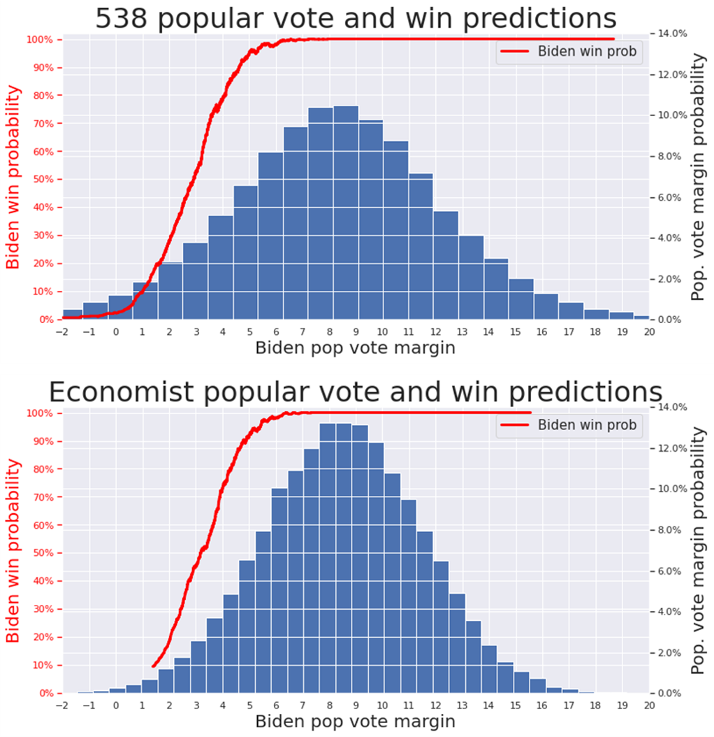
So, given all of the above, how much do these models differ? Perhaps surprisingy, the answer is “not by much”. To understand how they differ, I plotted for both models the following:

1. The histogram of Biden’s popular vote margin
2. The probability of Biden to win conditioned on a particular margin

Much of the methodological difference, including the issue of pairwise correlations, should manifest in 2, but eyeballing it, they don’t seem to differ that much. It seems that conditioned on a particular margin, both models give Biden similar probability to win. (In particular both models think that 3% margin is about 50/50, while 4% margin gives Biden about 80/20 chance). The main difference is actually in the first part of estimating the popular vote margin – 538 is more “conservative” and has fatter tails.

If you want to check my data, see if I have a bug, or try your own analysis, you can use this colab notebook.

“Make your own needle”

Another applications for such models is to help us adjust the priors as new information comes in. For example, it’s possible that Florida, North Carolina and Texas will report results early. If Biden loses one of these states, should we adjust our estimate of win probability significantly? It turns out that the answer depends on by how much he loses.

The following graphs show the updated win probability conditioned on a particular margin in a state. We see that winning or losing Florida, North Carolina, and Texas on their own doesn’t make much difference to the probability – it’s all about the margin. In contrast, losing Pennsylvania’s 20 electoral votes will make a significant difference to Biden’s chances.

(The non monotonicity is simply a side effect of having a finite number of simulation runs and would disappear in the limit.)