Quantum Approximate Optimization Algorithm and Applications

Motivation


Quantum computers have demonstrated great potential for solving certain problems more efficiently than their classical counterpart. Algorithms based on the quantum Fourier transform (QFT) such as Shor’s algorithm offer an exponential speed-up, while amplitude-amplification algorithms such as Grover’s search algorithm provide us with a polynomial speedup. The concept of “quantum supremacy” (quantum computers outperforming classical computers) has been explored for three general groups of problems:

  1. Structured problems, such as factoring and discrete logarithm. Out quantum computer takes advantage of the structure of these classes of problems to offer an exponential speedup compared to the best known classical alternative. While these speedups are the most promising, they require a large number of resources and are cannot be feasibly implemented in the near future.
  2. Quantum Simulations, originally proposed by Richard Feynman in the late 80s was thought to be the first motivation behind exploring quantum computation. Due to the fact that the space of all possible states of the system scales exponentially with the addition of a new element (eg. an atom), complex systems are very difficult to simulate classically. It has been shown that we can use a quantum computer to tackle interesting problems in quantum chemistry and chemical engineering. Furthermore, there are results on sampling the output of random quantum circuits which have been used for “quantum supremacy experiments”.
  3. General constraint satisfaction and optimization problems. Since these problems are NP-hard it is widely believed that we cannot gain an exponential speedup using a quantum computer, however, we can obtain quadratic speedup but utilizing a variation of Grover’s algorithm.

While these quantum algorithms are very exciting, they are beyond the capabilities of our near-term quantum computers; for example, any useful application of Shor’s factoring algorithm requires anywhere between tens of thousands to millions of qubits with error correction compared to quantum devices with hundreds of qubits that we might have available in the next few years.

Recently there has been increasing interest in hybrid classical-quantum algorithms among the community. The general idea behind this approach is to supplement the noisy intermediate-scale quantum (NISQ) devices with classical computers. In this blog post, we discuss the Quantum Approximate Optimization Algorithm (QAOA), which is a hybrid algorithm, alongside some of its applications.

Introduction

QAOA is used for optimizing combinatorial problems. Let’s assume a problem with n bits and m clauses. Each clause is a constraint on a subset of the bits which satisfies a certain assignment. We can define a cost function as follows:

C(z)=\sum_{\alpha=1}^m C_\alpha (z)

where z=z_1z_2...z_n is the bit string. In this article we consider a minimization problem, therefore we want C_\alpha(z)=0 if z satisfies clause \alpha and 1 otherwise. Note that in the case of a maximization problem we only need to switch the value assigned to a satisfactory clause to 1. Our objective is to find a (qu)bit string that minimizes (or maximizes) our cost function.

At a higher level, we start with a quantum state in a uniform superposition of all possible inputs z. This can be accomplished with n qubits which span a space of size 2^n. Our goal is to come up with a series of operations that would evolve our initial quantum state into a superposition of states in which the valid solutions would have a significantly higher probability than other states. In manner, upon sampling the quantum state we are likely to get the correct solution with high probability. QAOA uses the cost function to construct a set of operations that would be able to efficiently map the unifrom superposition state into the desired quantum state. These operators involve single qubits rotations around the x-axis, and multiqubit rotations around the z-axis of our qubits.

Now let’s discuss the details of QAOA. For this algorithm we assume that our quantum computer works in the computation basis of \left |0 \right > , \left | 1 \right > . We start by setting our initial state to a uniform superposition over computational basis states:

\left |s \right > = \frac{1}{\sqrt{2^n}}\sum_{z \in \{0,1\}^n} \left |z \right >

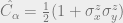
Next, we define a unitary operator using the cost function as follows:

U(\hat{C},\gamma) = e^{i\gamma \hat{C}}= \prod_{\alpha = 1}^m e^{-i\gamma \hat{C}_\alpha} 

Here we convert every clause C_\alpha to a Hamiltonian \hat{C_\alpha} consisting of Pauli Z ($\sigma^z$) operators. Just as a review, the two Pauli operators (X and Z) used in this blog post are representated as follows:

\sigma^x = \begin{pmatrix}    0 & 1 \\    1 & 0 \\\end{pmatrix} \: \: \: \:  \sigma^z = \begin{pmatrix}    1 & 0 \\    0 & -1 \\\end{pmatrix}

For example if C_\alpha=x \oplus y we can map the clause to \hat{C_\alpha}=\frac{1}{2}(1+\sigma^z_x \sigma^z_y) for a minimization problem. If x=\left |0 \right >   , then \sigma^z_x will return a value of 1, and if x=\left |1 \right > the operator will return -1. The same applies to qubit y as well. Therefore it is not hard to see that if x and y have the same value, then the operator \hat{C_\alpha} as defined above will result in a 1, and it’ll result in 0 otherwise. Furthermore, since \hat{C} has integer eigenvalues we can restrict the angle \gamma to lie in [0,2\pi].

Next, we define the admixing Hamiltonian:

B=\sum_{j=1}^n \sigma^x_j

and use it to define a unitary operator which consists of a product of commuting one qubit operations:
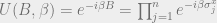
U(B,\beta) = e^{-i\beta B}= \prod_{j=1}^n e^{-i \beta \sigma_j^x}  

where \beta \in [0,\pi]. It’s easy to see that U(\Hat{C},\gamma) couples 2 or more qubits, while U(B,\beta) performs a single qubit rotation on the qubits in our system. Using these unitaries and our initial state we define a QAOA angle-dependent “ansatz” state as follows:

\left |  \boldsymbol{\gamma},\boldsymbol{\beta} \right >= U(B,\beta_p)U(\Hat{C},\gamma_p)...U(B,\beta_1)U(\Hat{C},\gamma_1) \left |s \right >

Here p\geq 1 is the “depth” of our QAOA circuit, and \boldsymbol{\gamma}=(\gamma_p,...,\gamma_1), \boldsymbol{\beta}=(\beta_p,...,\beta_1) are each a vector of length p controlling the angles for each layer. In the worst case scenario this state can be produce by a quantum circuit of depth mp+p, however by taking advantage of the structure of the instance we can further reduce the number of layers required. Let F_p be the expectation of \hat{C} in our ansatz:

F_p(\boldsymbol{\gamma},\boldsymbol{\beta})=\left < \boldsymbol{\gamma},\boldsymbol{\beta} \right | \hat{C} \left | \boldsymbol{\gamma},\boldsymbol{\beta} \right >

and let M_p be the minimum of F_p over angles,

M_p=\min_{\boldsymbol{\gamma},\boldsymbol{\beta}} F_p(\boldsymbol{\gamma},\boldsymbol{\beta}).

Note that minimization at p-1 layers can be viewed as a constrained minimization at p layers, therefore

M_p \leq M_{p-1}

Using an adiabatic approach [1] We can show that

\lim_{p \rightarrow \infty} M_p = \min_z C(z)

Based on these results our QAOA algorithm will look like the following:

  •  c: pick a p
  • c: choose a set of angles (\Vec{\gamma}_0,\Vec{\beta}_0)
  • q: prepare \left | \Vec{\gamma},\Vec{\beta} \right >  
  • q: compute F_p
  • c: perform gradient descend/ascend on F_p and get a new set of angles (\Vec{\gamma},\Vec{\beta})
  • repeat from step 3 till convergence
  • report the measurement result of \left | \Vec{\gamma},\Vec{\beta} \right >   in computational basis

If p does not asymptotically grow with n F_p(\Vec{\gamma},\Vec{\beta}) can be efficiently computed in O(m^2+mn)

Application: MaxCut

In this section we apply the QAOA algorithm to the MaxCut problem with bounded degree. MaxCut is an NP-hard problem that asks for a subset S of the vertex set such that the number of edges between S and the complementary subset is as large as possible. While QAOA does not offer a theoretical guarantee to solve MaxCut in polynomial time, it offers a path to utilizing NISQ devices for tackling such optimization problems and discuss patterns in such problems that can be used for reducing the number of steps required.

For this section, let’s assume p=O(1), and we have a graph with n vertices and an edge set \{<jk>\} of size m. We can construct a cost function to be maximized as follows:

C = \sum_{<jk>} C_{<jk>}

C_{<jk>} = \frac{1}{2} (1-\sigma^z_j \sigma^z_k)

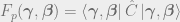
We can the compute the angle dependent cost of our ansatz as follows:

F_p(\Vec{\gamma},\Vec{\beta})=\sum_{<jk>}\left <{s} \right | U^\dagger(C,\gamma_1)...U^\dagger(B,\beta_p) C_{<jk>}U(B,\beta_p) ... U(C,\gamma_1) \left |s \right >

Let’s consider the operation associated with some edge <jk>:

U ^\dagger(C,\gamma_1)...U^\dagger(B,\beta_p) C_{<jk>}U(B,\beta_p) ... U(C,\gamma_1)

Since QAOA consists of local operations, we may take advantage by thinking about the problem in terms of subproblems (or subgraphs) involving certain nodes. This property will allow us to simplify our clauses even further depending on the desired depth p of our quantum circuit, therefore decreasing the amount of resources necessary to implement the algorithm.

The operator C_{<jk>} includes qubits (nodes) j and k, therefore the sequence of operators above will only involve qubits that are at most distance p away from qubits j and k. Let’s consider the example of p=1:

\rightarrow U^\dagger(C,\gamma_1)e^{i\beta_1(\sigma^x_j + \sigma^x_k)} C_{<jk>} e^{-i\beta_1(\sigma^x_j + \sigma^x_k)} U(C,\gamma_1).

It’s easy to see that any factor of U(C,\gamma_1) that does not depend on j or k will commute through and cancel out. Since the degree is bounded, each subgraph contains a number of qubits that is independent of n, which allows for the evaluation of F_p in terms of subsystems of size independent of n.

For an subgraph G define:

C_G=\sum_{<l l^\prime>} C_{<l l^\prime>}  \: \: \: \: U(C_G,\gamma)=e^{-i \gamma C_G}

B_G = \sum_{j \in G} \sigma^x_j  \: \: \: \: U(B_G,\beta) = e^{-i \beta B_G}

\left | s,G \right >   = \prod_{l \in G} \left |+ \right > _l

We can define our total cost as a sum over the cost of each subgraph:

f_g(\Vec{\gamma},\Vec{\beta})=\left < s,g(j,k) \right |  U ^\dagger(C_{g(j,k)},\gamma_1)...U^\dagger(B_{g(j,k)},\beta_p) C_{<jk>}U(B_{g(j,k)},\beta_p) ... U(C_{g(j,k)},\gamma_1) \left |s,g(j,k) \right >

where g(j,k) is a subgraph of type g and “…” is used to omit the sequence of angle depending unitaries constructed using the elements of \Vec{\gamma} and \Vec{\beta}. F_p is then

F_p(\Vec{\gamma},\Vec{\beta})=\sum_g w_g f_g(\Vec{\gamma},\Vec{\beta})

where w_g is the number of occurrence of the subgraph g in the original edge sum. The function f_g does not depend on n and m, and the only dependence on these variables comes through the weights w_g from the original graph. The maximum number of qubits that can appear in our sequence of operators comes when the subgraph is a tree. For a graph with maximum degree v, the number of qubits in this tree is

q_{tree}=2[\frac{(v-1)^{p+1}-1}{(v-1)-1}]

(or 2p+2 if v=2), which is independent of n and m. Therefore we can see that for constant p F_p can be efficiently computed.

Next, let’s consider the spread of C measured in the state \left | \Vec{\gamma},\Vec{\beta} \right >  .

\left <\Vec{\gamma},\Vec{\beta} \right | C^2\left |\Vec{\gamma},\Vec{\beta}\right >  -\left < \Vec{\gamma},\Vec{\beta} \right | C \left | \Vec{\gamma},\Vec{\beta} \right > ^2 \leq 2[\frac{(v-1)^{2p+2}-1}{(v-1)-1}].m

For fixed v and p we see that the standard deviation of C(z) is upper-bounded by O(\sqrt{m}). Using this fact and the appropriate probability bounds we can see that the result of measuring the cost function of the state \left | \vec{\gamma_{opt}},vec{\beta_{opt}} \right >   will be very close to the intended value of F_p(\vec{\gamma_{opt}},\vec{\beta_{opt}}) which bounds the uncertainty present in quantum measurement.

Bibliography

[1] E. Farhi, J. Goldstone, and S. Gutmann, “A Quantum Approximate Optimization Algorithm,” 2014.

[2] J. S. Otterbach, et. al, “Unsupervised Machine Learning on a Hybrid Quantum Computer,” 2017.

Leave a comment