By Abhijit Mudigonda, Richard Wang, and Lisa Yang

This is part of a series of blog posts for CS 229r: Physics and Computation. In this post, we will talk about progress made towards resolving the quantum PCP conjecture. We’ll briefly talk about the progression from the quantum PCP conjecture to the NLTS conjecture to the NLETS theorem, and then settle on providing a proof of the NLETS theorem. This new proof, due to Nirkhe, Vazirani, and Yuen, makes it clear that the Hamiltonian family used to resolve the NLETS theorem cannot help us in resolving the NLTS conjecture.

Introduction

We are all too familiar with NP problems. Consider now an upgrade to NP problems, where an omniscient prover (we’ll call this prover Merlin) can send a polynomial-sized proof to a BPP (bounded-error probabilistic polynomial-time) verifier (and we’ll call this verifier Arthur). Now, we have more decision problems in another complexity class, MA (Merlin-Arthur). Consider again, the analogue in the quantum realm where now the prover sends over qubits instead and the verifier is in BQP (bounded-error quantum polynomial-time). And now we have QMA (quantum Merlin-Arthur).

We can show that there is a hierarchy to these classes, where NP $\subseteq$ MA $\subseteq$ QMA.

Our goal is to talk about progress towards a quantum PCP theorem (and since nobody has proved it in the positive or negative, we’ll refer to it as a quantum PCP conjecture for now), so it might be a good idea to first talk about the PCP theorem. Suppose we take a Boolean formula, and we want to verify that it is satisfiable. Then someone comes along and presents us with a certificate — in this case, a satisfying assignment — and we can check in polynomial time that either this is indeed a satisfying assignment to the formula (a correct certificate) or it is not (an incorrect certificate).

But this requires that we check the entire certificate that is presented to us. Now, in comes the PCP Theorem (for probabilistically checkable proofs), which tells us that a certificate can be presented to us such that we can read a constant number of bits from the certificate, and have two things guaranteed: one, if this certificate is correct, then we will never think that it is incorrect even if we are not reading the entire certificate, and two, if we are presented with an incorrect certificate, we will reject it with high probability [1].

In short, one formulation of the PCP theorem tells us that, puzzingly, we might not need to read the entirety of a proof in order to be convinced with high probability that it is a good proof or a bad proof. But a natural question arises, which is to ask: is there a quantum analogue of the PCP theorem?

Progress

The answer is, we’re still not sure. But to make progress towards resolving this question, we will present the work of Nirkhe, Vazirani, and Yuen in providing an alternate proof of an earlier result of Eldar and Harrow on the NLETS theorem.

Before we state the quantum PCP conjecture, it would be helpful to review information about local Hamiltonians and the $k$ -local Hamiltonian problem. A previous blog post by Ben Edelman covers these topics. Now, let’s state the quantum PCP conjecture:

(Quantum PCP Conjecture): It is QMA-hard to decide whether a given local Hamiltonian $H = H_{1} + ... + H_{m}$ (where each $||H_{i}|| \leq 1$ ) has ground state energy at most $a$ or at least $b$ when $b-a \geq c||H||$ for some universal constant $c > 0$ .

Recall that MAX- $k$ -SAT being NP-hard corresponds to the $k$ -local Hamiltonian problem being QMA-hard when $b-a \geq 1/poly(n)$ . (We can refer to Theorem 4.1 in these scribed notes of Ryan O’Donnell’s lecture, and more specifically to Kempe-Kitaev-Regev’s original paper for proof of this fact.) The quantum PCP conjecture asks if this is still the case when the gap is $c||H||$ .

Going back to the PCP theorem, an implication of the PCP theorem is that it is NP-hard to approximate certain problems to within some factor. Just like its classical analogue, the qPCP conjecture can be seen as stating that it is QMA-hard to approximate the ground state energy to a factor better than $c||H||$ .

Reformulation: NLTS conjecture

Let’s make the observation that, taking $a$ to be the ground state energy, the qPCP conjecture sort of says that there exists a family of Hamiltonians for which there is no trivial state (a state generated by a low depth circuit) such that the energy is at most $c||H||$ above the ground state energy.

Freedman and Hastings came up with an easier goal called the No Low-Energy Trivial States conjecture, or NLTS conjecture. We expect that ground states of local Hamiltonians are sufficiently hard to describe (if NP $\neq$ QMA). So low-energy states might not be generated by a quantum circuit of constant depth. More formally:

(NLTS Conjecture): There exists a universal constant $\epsilon > 0$ and a family of local Hamiltonians $\{H^{(n)}\}_{n=1}^{\infty}$ where $H^{(n)}$ acts on $n$ particles and consists of $m_{n}$ local terms, s.t. any family of states $\{|\psi_{n}\rangle\}$ satisfying $\langle \psi_{n} | H^{(n)} | \psi_{n}\rangle \leq \epsilon||H^{(n)}|| + \lambda_{min}(H^{(n)})$ requires circuit depth that grows faster than any constant.

To reiterate, if we did have such a family of NLTS Hamiltonians, then it we wouldn’t be able to give “easy proofs” for the minimal energy of a Hamiltonian, because we couldn’t just give a small circuit which produced a low energy state.

Progress: NLETS theorem

$\epsilon$ -error states are states that differ from the ground state in at most $\epsilon n$ qubits. Now, consider $\epsilon$ -error states (which “agree” with the ground state on most qubits). Then for bounded-degree local Hamiltonians (analogously in the classical case, those where each variable participates in a bounded number of clauses), these states are also low energy. So any theorem which applies to low energy states (such as the NLTS conjecture), should also apply to states with $\epsilon$ -error (as in the NLETS theorem).

To define low-error states more formally:

Definition 2.1 ( $\epsilon$ -error states): Let $\rho, \sigma \in D((\mathbb{C}^{d})^{\otimes n})$ (the space of positive semidefinite operators of trace norm equal to 1 on $(\mathbb{C}^{d})^{\otimes n}$ ). Let $H$ be a local Hamiltonian acting on $(\mathbb{C}^{d})^{\otimes n}$ . Then:

$\sigma$ is an $\epsilon$ -error state of $\rho$ if $\exists S \subseteq [n]$ of size at most $\epsilon n$ s.t. $\text{Tr}_{S}(\rho) = \text{Tr}_{S}(\sigma)$ .
$\sigma$ is an $\epsilon$ -error state for $H$ if $\exists \rho$ s.t. $\text{Tr}(H\rho) = \lambda_{min}(H)$ and $\sigma$ is an $\epsilon$ -error state for $\rho$ .

Here, see that $\text{Tr}_{S}$ is just the partial trace on some subset of integers $S$ , like we’re tracing out or “disregarding” some subset of $n$ qubits.

In 2017, Eldar and Harrow showed the following result which is the NLETS theorem.

Theorem 1 (NLETS Theorem): There exists a family of 16-local Hamiltonians $\{H^{(n)}\}$ s.t. any family of $\epsilon$ -error states $\{|\Phi_{n}\rangle\}$ for $\{H^{(n)}\}$ requires circuit depth $\Omega(\log n)$ where $\epsilon = 10^{-9}$ .

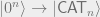
In the next two sections, we will provide background for an alternate proof of the NLETS theorem due to Nirkhe, Vazirani, and Yuen. After this, we will explain why the proof of NLETS cannot be used to prove NLTS, since the local Hamiltonian family we construct for NLETS can be linearized. Nirkhe, Vazirani, and Yuen’s proof of NLETS makes use of the Feynman-Kitaev clock Hamiltonian corresponding to the circuit generating the cat state (Eldar and Harrow make use of the Tillich-Zemor hypergraph product construction; refer to section 8 of their paper). What is this circuit? It is this one:

First, we apply the Hadamard gate (drawn as $\boxed{H}$ ) which maps the first qubit $|0\rangle \rightarrow \frac{|0\rangle + |1\rangle}{\sqrt{2}}$ . Then we can think of the CNOT gates (drawn as $\bullet-\oplus$ ) as propagating whatever happens to the first qubit to the rest of the qubits. If we had the first qubit mapping to 0, then the rest of the qubits map to 0, and likewise for 1. This generates the cat state $|\textsf{CAT}_{n}\rangle = \frac{|0\rangle^{\otimes n} + |1\rangle^{\otimes n}}{\sqrt{2}}$ , which is highly entangled.

Why do we want a highly entangled state? Roughly our intuition for using the cat state is this: if the ground state of a Hamiltonian is highly entangled, then any quantum circuit which generates it has non-trivial depth. So if our goal is to show the existence of local Hamiltonians which have low energy or low error states that need deep circuits to generate, it makes sense to use a highly entangled state like the cat state.

Quantum circuits

(We’ll write that the state of a qudit – a generalization of a qubit to more than two dimensions, and in this case $q$ dimensions – is a vector in $\mathbb{C}^{q}$ . In our diagram above, we’ll see 4 qudits, labelled appropriately.)

Let’s briefly cover the definitions for the quantum circuits we’ll be using.

Let $U$ be a unitary operator acting on a system of $n$ qudits (in other words, acting on $(\mathbb{C}^{q})^{\otimes n}$ ), where $U = U_{m} \hdots U_{1}$ . Here, each $U_{i}$ is a unitary operator (a gate) acting on at most two qudits, and $U$ is a product of $m$ such operators.

If there exists a partition $U$ into products of non-overlapping two-qudit unitaries (we call these layers and denote them as $L_{i} = \bigotimes_{j}U_{ij}$ , where each $U_{j}$ here is in layer $L_{i}$ ) such that $U = L_{d} \hdots L_{1}$ then we say $U$ has $d$ layers.

In other words, $U$ has size $m$ and circuit depth $d$ .

Lightcones, effect zones, shadow zones

Consider $U = L_{d} \hdots L_{1}$ and $A$ an operator.

For $j < d$ define $K^{(j)}$ as the gates in layer $j$ whose supports overlap that of any gate in $K^{(j+1)}$ , …, $K^{(d)}$ or with $A$ .

Definition 3.1 (lightcone): The lightcone of $A$ with respect to $U$ is the union of $K^{(j)}$ : $K_{U} \triangleq \bigcup_{j} K^{(j)}$ .

So we can think of the lightcone as the set of gates spreading out of $A$ all the way to the first layer of the circuit. In our diagram, the lightcone of $A$ is the dash-dotted region. We have $K^{(3)} = \varnothing$ , $K^{(2)} = \{U_{21}\}$ , and $K^{(1)} = \{U_{11}, U_{12}\}$ .

We also want a definition for what comes back from the lightcone: the set of gates from the first layer (the widest part of the cone) back to the last layer.

Define $E^{(1)} = K^{(1)}$ . For $j \geq 2$ , let $E^{(j)}$ be the set of gates whose supports overlap with any gate in $E^{(j-1)}$ .

Definition 3.2 (effect zone): The effect zone of $A$ with respect to $U$ is the union $E_{U}(A) \triangleq \bigcup_{j} E^{(j)}$ .

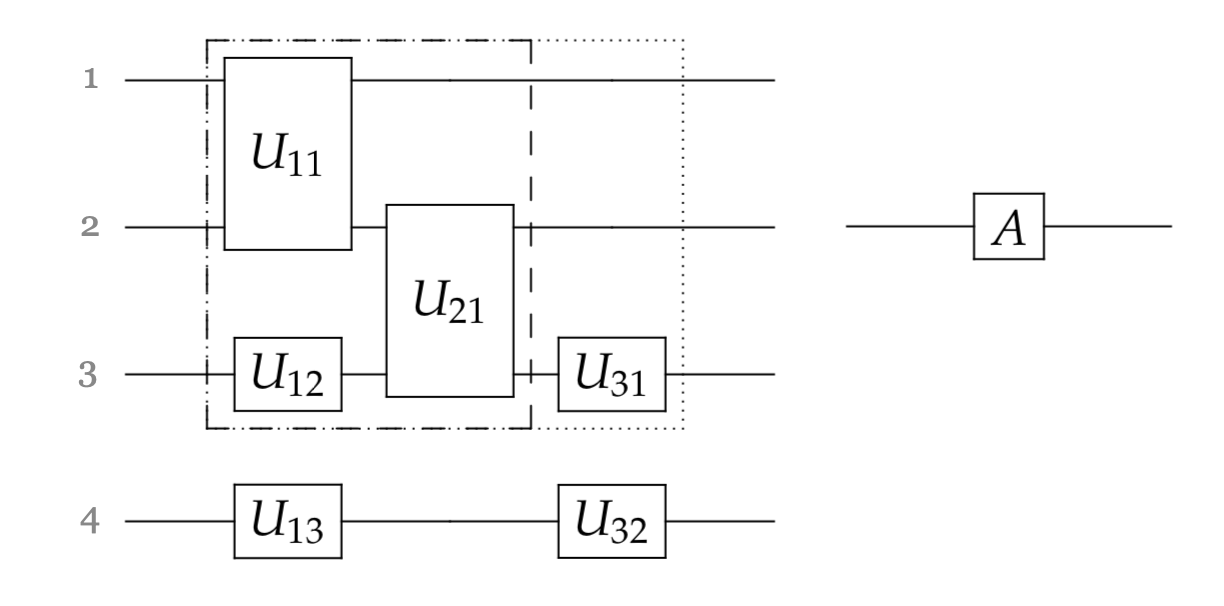
In our diagram, see that $E^{(1)} = \{U_{11}, U_{12}\}$ , $E^{(2)} = \{U_{21}\}$ , and $E^{(3)} = \{U_{31}\}$ . The effect zone of $A$ is the dotted region.

Definition 3.3 (shadow of the effect zone): The shadow of the effect zone $W_{U}(A)$ of $A$ with respect to $U$ is the set of qudits acted on by the gates in the effect zone.

In our diagram, the first three qudits are effected by gates in the effect zone. So $W_{U}(A) = \{1, 2, 3\}$ .

Given all of these definitions, we make the following claim which will be important later, in a proof of a generalization of NLETS.

Claim 3.1 (Disjoint lightcones): Let $U$ be a circuit and $A, B$ operators. If the qudits $B$ acts on are disjoint from $W_{U}(A)$ , then the lightcones of $A$ and $B$ in $U$ are disjoint.

Toward the Feynman-Kitaev clock

Now we’ll give some definitions that will become necessary when we make use of the Feynman-Kitaev Hamiltonian in our later proofs.

Let’s define a unary clock. It will basically help us determine whatever happened at any time little $t$ along the total time big $T$ . Let $|\textsf{unary}(t, T)\rangle = |0\rangle^{\otimes(T-t)} \otimes |1\rangle^{\otimes t}$ . For our purposes today, we won’t worry about higher dimensional clocks. So we’ll write $|\textsf{clock}_{k}(t, T)\rangle$ , but we’ll really only consider the case where $k = 1$ , which corresponds to $|\textsf{unary}(t, T)\rangle$ . For simplicity’s sake, we will henceforth just write $|\textsf{unary}(t)\rangle$ .

Our goal is to construct something a little similar to the tableaux in the Cook-Levin theorem, so we also want to define a history state:

Definition 4.1 (History state): Let $C$ be a quantum circuit that acts on a witness register and an ancilla register. Let $C_{1}, ..., C_{T}$ denote the sequence of two-local gates in $C$ . Then for all $k \in \mathbb{N}$ , a state $|\Psi\rangle$ is a $k$ -dimensional history state of $C$ if:

$\begin{aligned}|\Psi\rangle = \frac{1}{\sqrt{T+1}}\sum_{t=0}^{T}|\textsf{clock}_{k}(t, T)\rangle \otimes |\psi_{t}\rangle\end{aligned}$

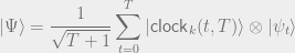
where we have the clock state to keep track of time and $\psi_{t}$ is some state such that $|\psi_{t}\rangle = C_{t}|\psi_{t-1}\rangle$ and $|\psi_{0}\rangle = |\xi\rangle_{witness} \otimes |0\rangle_{ancilla}$ . With this construction, we should be able to make a measurement to get back the state at time $t$ .

Proof of NLETS

We provide a proof of (a simplified case of) the NLETS theorem proved by Nirkhe, Vazirani, and Yuen in [2].

Theorem 2 (NLETS): There exists a family of $3$ -local Hamiltonians $\{H^{(n)}\}$ on a line (Each Hamiltonian $H^{(n)}$ can be defined on $n$ particles arranged on a line such that each local Hamiltonian acts on a particle and its two neighbors) such that for all $n \in \mathbb{N}$ , the circuit depth of any $\epsilon$ -error ground state for $H^{(n)}$ is at least logarithmic in $n$ .

First, we’ll show the circuit lower bound. Then we’ll explain why these Hamiltonians can act on particles on a line and what this implies about the potential of these techniques for proving NLTS.

Proof: We will use the Feynman-Kitaev clock construction to construct a $5$ -local Hamiltonian $\mathcal{H}^{(n)}$ for the circuit $C_n$ : $|0^n\rangle \to |\textsf{CAT}_n\rangle$ .

Fix $n \in \mathbb{N}$ and let $C_n$ have size $T$ . The Hamiltonian $\mathcal{H}$ acts on $T+n$ qubits and consists of several local terms depending on $C_n$ :

$\begin{aligned}\mathcal{H} = H_{in} + \sum_{t=1}^T H_t + H_{out} + H_{stab}\end{aligned}$

We can think of a $T+n$ qubit state as representing a $T$ step computation on $n$ qubits (i.e. for each time $t \in [0,T]$ , we have a $n$ bit computation state $\textsf{state}_t$ of $C_n$ ). Intuitively, a $T+n$ qubit state has energy $0$ with respect to $\mathcal{H}$ iff it is the history state of $C_n$ . This is because $H_{in}$ checks that at time $t=0$ , $\textsf{state}_0$ consists of the input $|0\rangle^n$ to $C_n$ . Each $H_t$ checks that $\textsf{state}_{t}$ proceed correctly from $\textsf{state}_{t-1}$ (i.e. that the $t$ th gate of $C_n$ is applied correctly). Then $H_{out}$ checks that at time $t=T$ , the output is $1$ . Finally, $H_{stab}$ checks that the $T+n$ qubit state is a superposition only over states where the first $T$ qubits represent “correct times” (i.e. a unary clock state where time $t$ is represented by $T-t$ zeros followed by $t$ ones).

Therefore, $\mathcal{H}$ has a unique ground state, the history state of $C_n|0^n\rangle$ , with energy $0$ :

$\begin{aligned}|\Psi\rangle = \frac{1}{\sqrt{n+1}}\sum_{t=0}^n |\textsf{unary}(t)\rangle\otimes |\psi_t\rangle = \frac{1}{\sqrt{n+1}}\sum_{t=0}^n |\textsf{unary}(t)\rangle\otimes|\textsf{CAT}_{t}\rangle\otimes |0\rangle^{\otimes (n-t)}\end{aligned}$

Later we will show how to transform $\mathcal{H}$ into a Hamiltonian $H$ on $n$ qutrits on a line. Intuitively, the structure of $C_n$ allows us to fuse the $T=n$ time qubits and $n$ state qubits and represent unused state qubits by $2$ . For the Hamiltonian $H$ , the ground state becomes

$\begin{aligned}|\Psi\rangle = \frac{1}{\sqrt{n+1}}\sum_{t=0}^n |\psi_t\rangle = \sum_{t=0}^n |\textsf{CAT}_{t}\rangle\otimes|2\rangle^{\otimes(n-t)}\end{aligned}$

For the rest of this proof, we work with respect to $H$ .

Let $\sigma$ be an $\epsilon$ -error state and let $S \subseteq [n]$ be the subset of qutrits such that $\text{Tr}_S(\sigma) = \text{Tr}_S(|\Psi\rangle\langle\Psi|)$ . We define two projection operators which, when applied to $\sigma$ alone, produce nontrivial measurements, but when applied to $\sigma$ together, produce trivial measurements.

Definition 5.1: For any $i\in[n]$ , the projection operator

$\begin{aligned}A_i = |0\rangle\langle 0|_i \end{aligned}$

projects onto the subspace spanned by $0$ on the $i$ th qutrit.

For any $j\in[n]$ , the projection operator

$\begin{aligned} B_j = |1\rangle\langle 1|_i\end{aligned}$

projects onto the subspace spanned by $1$ on the $j$ th qutrit.

Claim 5.1: For $i\not\in S$ , $\text{Tr}(A_i\sigma) = \frac{1}{2} + \frac{-i}{2(n+1)}$ . For $j\not\in S$ , $\text{Tr}(B_j\sigma) = \frac{1}{2} + \frac{-j}{2(n+1)}$ . Note that these values are positive for any $i,j\in [n]$ .

Proof: If $i \not\in S$ , then measurements on the $i$ th qutrit are the same for $\sigma$ and $|\Psi\rangle\langle\Psi|$ .

$\begin{aligned} \text{Tr}(A_i\sigma) &= \text{Tr}(A_i|\Psi\rangle\langle\Psi|)\\ &= \text{Tr}\left(A_i \frac{1}{n+1}\sum_{t,t'}|\psi_t\rangle\langle\psi_{t'}|\right)\\ &= \frac{1}{n+1}\sum_{t,t'} \text{Tr}(A_i|\psi_t\rangle\langle\psi_{t'}|) \end{aligned}$

If $t=t'$ , then any $n$ qutrit pure state cannot have nonzero weight in both $\psi_t$ and $\psi_{t'}$ (every pure state ends in some number of $2$ s which tells which $\psi_t$ (if any) it can be a part of). Therefore,

$\begin{aligned} \text{Tr}(A_i\sigma) = \frac{1}{n+1}\sum_{t} \text{Tr}(A_i|\psi_t\rangle\langle\psi_{t}|) = \frac{1}{n+1}\sum_t \langle \psi_t|A_i|\psi_t\rangle \enspace. \end{aligned}$

If $i \le t$ , then projecting onto the $i$ th qutrit gives $0$ with probability $1/2$ . Therefore, $\text{Tr}(A_i\sigma) = \frac{1}{n+1}\left(\frac{n-i+1}{2}\right) = \frac{1}{2} + \frac{-i}{2(n+1)}$ .

Similarly, $\text{Tr}(B_j\sigma) = \frac{1}{2} + \frac{-j}{2(n+1)}$ . $\square$

Claim 5.2: For $i,j \not\in S$ such that $i < j$ , $\text{Tr}(A_i \otimes B_j \sigma) = 0$ .

Proof: As before, we can calculate

$\begin{aligned} \text{Tr}(A_i \otimes B_j \sigma) &= \text{Tr}(A_i \otimes B_j |\Psi\rangle \langle\Psi|) = \frac{1}{n+1}\sum_t \langle\psi_t|A_i\otimes B_j|\psi_t\rangle \end{aligned}$

If $j > t$ , then the $j$ th qutrit of $\psi_t$ is $2$ so $B_j|\psi_t\rangle = 0$ . If $j \le t$ , then $A_i \otimes B_j|\psi_t\rangle = 0$ because the first $t$ qutrits of $|\psi_t\rangle$ contain the $|\textsf{CAT}_{t}\rangle$ state so under any measurement, the $i$ and $j$ th qutrits must be the same. $\square$

Now we use these claims to prove a circuit lower bound. Let $U$ be a circuit generating (a state with density matrix) $\sigma$ . Let $d$ be the depth of $U$ .

Consider some $i\not\in S$ . For any operator acting on the $i$ th qutrit, its lightcone consists of at most $2^d$ gates so its effect zone consists of at most $2^{2d}$ gates which act on at most $2^{2d+1}$ qudits (called the shadow of the effect zone).

Assume towards contradiction that $2^{2d+1} < n-\epsilon n$ . Then the shadow of any operator acting only on the $i$ th qutrit has size at most $2^{2d+1} \le n - |S|$ since $|S| \le \epsilon n$ . So there is some $j$ outside of the shadow which is in the complement of $S$ . By Claim 3.1, we have found two indices $i,j$ such that any pair of operators acting on $i$ and $j$ have disjoint lightcones in $U$ . WLOG let $i < j$ . The lightcones of $A_i,B_j$ are disjoint which implies $\begin{aligned}\text{Tr}(A_i \otimes B_j \sigma) = \text{Tr}(A_i \sigma)\cdot\text{Tr}(B_j \sigma).\end{aligned}$

By the two claims above, we get a contradiction.

Therefore, $2^{2d+1} \ge n-\epsilon n$ . We can take any constant epsilon: letting $\epsilon = 1/2$ , we get

$\begin{aligned}d \ge \frac{1}{2}\left(\log \frac{n}{2} - 1\right)\end{aligned}$

$\square$

This analysis relies crucially on the fact that any $\epsilon$ -error state matches the groundstate on most qudits. However, NLTS is concerned with states which may differ from the groundstate on many qudits, as long as they have low energy.

Remark 2.1: The paper of Nirkhe, Vazirani, and Yuen [2] actually proves more:

A more general lower bound: logarithmic lower bound on the circuit depth of any $\delta$ -approximate ( $\delta$ far in L1 norm) $\epsilon$ -noisy state (probability distribution over $\epsilon$ -error states).

Assuming QCMA $\neq$ QMA (QCMA takes a $m$ bit witness string instead of a $m$ qubit state as witness), they show a superpolynomial lower bound (on the circuit depth of any $\delta$ -approximate $\epsilon$ -noisy state).

“Approximate qLWC codes”, using techniques from their superpolynomial lower bound.

Back to NLTS – Tempering our Optimism

So far, we’ve shown a local Hamiltonian family for which all low-error (in “Hamming distance”) states require logarithmic quantum circuit depth to compute, thus resolving the NLETS conjecture. Now, let’s try to tie this back into the NLTS conjecture. Since it’s been a while, let’s recall the statement of the conjecture:

Conjecture (NLTS): There exists a universal constant $\epsilon > 0$ and a family of local Hamiltonians $\{H^{(n)}\}_{n=1}^{\infty}$ where $H^{(n)}$ acts on $n$ particles and consists of $m_{n}$ local terms, s.t. any family of states $\{|\psi_{n}\rangle\}$ satisfying $\langle \psi_{n} | H^{(n)} | \psi_{n}\rangle \leq \epsilon||H^{(n)}|| + \lambda_{min}(H^{(n)})$ requires circuit depth that grows faster than any constant.

In order to resolve the NLTS conjecture, it thus suffices to exhibit a local Hamiltonian family for which all low-energy states require logarithmic quantum circuit depth to compute. We might wonder if the local Hamiltonian family we used to resolve NLETS, which has “hard ground states”, might also have hard low-energy states. Unfortunately, as we shall show, this cannot be the case. We will start by showing that Hamiltonian families that lie on constant-dimensional lattices (in a sense that we will make precise momentarily) cannot possibly be used to resolve NLTS, and then show that the Hamiltonian family we used to prove NLTS can be linearized (made to lie on a one-dimensional lattice!).

The Woes of Constant-Dimensional Lattices

Definition 6.1: A local Hamiltonian $H$ acting on $n$ qubits is said to lie on a graph $G$ if there is an injection of qubits into vertices of the graph such that the set of qubits in any interaction term correspond to a connected component in the graph.

Theorem 2: If $(H^{(n)})$ is a local Hamiltonian family that lies on an $O(1)$ -dimensional lattice, then $(H^{(n)})$ has a family of low-energy states with low circuit complexity. In particular, if $H$ is a local Hamiltonian on a $d$ -dimensional lattice acting on $n$ qubits for large enough $n$ , then for any $\epsilon$ , there exists a state $|\psi\rangle$ that can be generated by a circuit of constant depth and such that $\langle \psi | H | \psi \rangle \leq H_0 + \epsilon ||H||$ where $H_0$ is the ground-state energy.

Proof: In what follows, we’ll omit some of the more annoying computational details in the interest of communicating the high-level idea.

Start by partitioning the $d$ -dimensional lattice (the one that $H^(n)$ lives on) into hypercubes of side length $L$ . We can “restrict” $H^{(n)}$ to a given hypercube (let’s call it $\rho$ ) by throwing away all local terms containing a qubit not in $\rho$ . This gives us a well-defined Hamiltonian $H_{\rho}$ on the qubits in $\rho$ . Define $|\phi_{\rho}\rangle$ to be the $L^d$ -qubit ground state of $H_{\rho}$ , and define

$\begin{aligned}|\phi\rangle := \bigotimes_{\text{hypercubes } \rho} |\phi_{\rho}\rangle\end{aligned}$

where $|\phi\rangle$ is an $n$ -qubit state. Each $|\phi_{\rho}\rangle$ can be generated by a circuit with at most $2^{L^d}$ gates, hence at most $2^{L^d}$ depth. Then, $|\phi\rangle$ can be generated by putting all of these individual circuits in parallel – this doesn’t violate any sort of no-cloning condition because the individual circuits act on disjoint sets of qubits. Therefore, $|\phi\rangle$ can be generated by a circuit of depth at most $2^{L^d}$ . $L$ and $d$ are both constants, so $|\phi\rangle$ can be generated by a constant-depth circuit.

We claim that, for the right choice of $L$ , $|\phi\rangle$ is also a low-energy state. Intuitively, this is true because $\phi$ can only be “worse” than a true ground state of $H^{(n)}$ on local Hamiltonian terms that do not lie entirely within a single hypercube (i.e. the boundary terms), and by choosing $L$ appropriately we can make this a vanishingly small fraction of the local terms of $H^{(n)}$ . Let’s work this out explicitly.

Each hypercube has surface area $2dL^{d-1}$ , and there are $n/L^d$ hypercubes in the lattice. Thus, the total number of qubits on boundaries is at most $2d\frac{n}{L}$ . The number of size $k$ -connected components containing a given point in a $d$ -dimensional lattice is a function of $k$ and $d$ . Both of these are constants. Therefore, the number of size $k$ -connected components containing a given vertex, and hence the number of local Hamiltonian terms containing a given qubit, is constant. Thus, the total number of violated local Hamiltonian terms is at most $O(\frac{n}{L})$ . Taking $L$ to be $\frac{1}{\epsilon}$ , we get the desired bound. Note that to be fully rigorous, we need to justify that the boundary terms don’t blow up the energy, but this is left as an exercise for the reader. $\square$

Linearizing the Hamiltonian

Now that we have shown that Hamiltonians that live on constant-dimensional lattices cannot be used to prove NLTS, we will put the final nail in the coffin by showing that our NLETS Hamiltonian (the Feynman-Kitaev clock Hamiltonian $\mathcal{H}$ on the circuit $C$ ) can be made to lie on a line (a $1$ -dimensional lattice). To do so, we will need to understand the details of $\mathcal{H}$ a bit better.

Proposition 6.1: $\mathcal{H}$ for the circuit $C$ is $5$ -local.

Proof: Recall that we defined

$\begin{aligned}\mathcal{H} := H_{in} + \sum_{t=1}^T H_t+ H_{stab}\end{aligned}$

Let’s go through the right-hand-side term-by-term. We will use $|\mathsf{time}(t)\rangle$ to denote the $t^{\text{th}}$ qubit of the time register and $|\mathsf{state}(s)\rangle$ to denote the $s^{\text{th}}$ qubit of the state register.

$H_{in}$ needs to serially access the qubit pairs $\begin{aligned}|\mathsf{time}(0)\rangle\otimes\textsf{state}(s) \end{aligned}$ for all $s$ and ensure that they are all set to $|0\rangle$ . Thus, $H_{in}$ is $2$ -local.
Each $H_t$ term needs to access the states $|\textsf{time}(t-1)\rangle, |\textsf{time}(t)\rangle, |\textsf{time}(t+1)\rangle, |\textsf{state}(s)\rangle$ , and $|\textsf{state}(t)\rangle$ and ensure that the state transitions are correct. Thus, $H_{t}$ is $5$ -local.
$H_{stab}$ needs to access the states $\begin{aligned}|\textsf{time}(t)\rangle \otimes |\textsf{time}(t+1)\rangle \end{aligned}$ and ensure that the progression of the time register is correct. Thus, $H_{stab}$ is $2$ -local. $\square$

Now, we follow an approach of [3] to embed $\mathcal{H}$ into a line.

Theorem 3: The Feynman-Kitaev clock Hamiltonian $H$ can be manipulated into a $3$ -local Hamiltonian acting on qutrits on a line.

Proof: Rather than having $\mathcal{H}$ act on $2n$ total qubits ( $n$ time qubits and $n$ state qubits), let’s fuse each $|\textsf{time}(i)\rangle$ and $|\textsf{state}(i)\rangle$ pair into a single qudit of dimension $4$ . If we view $\mathcal{H}$ as acting on the space of particles $|\textsf{time}(i)\rangle \otimes |\textsf{state}(i)\rangle$ , we observe that, following Proposition 6.1, each local term needs to check at most the particles corresponding to times $t-1$ , $t$ , and $t+1$ . Therefore, $\mathcal{H}$ is $3$ -local and on a line, as desired.

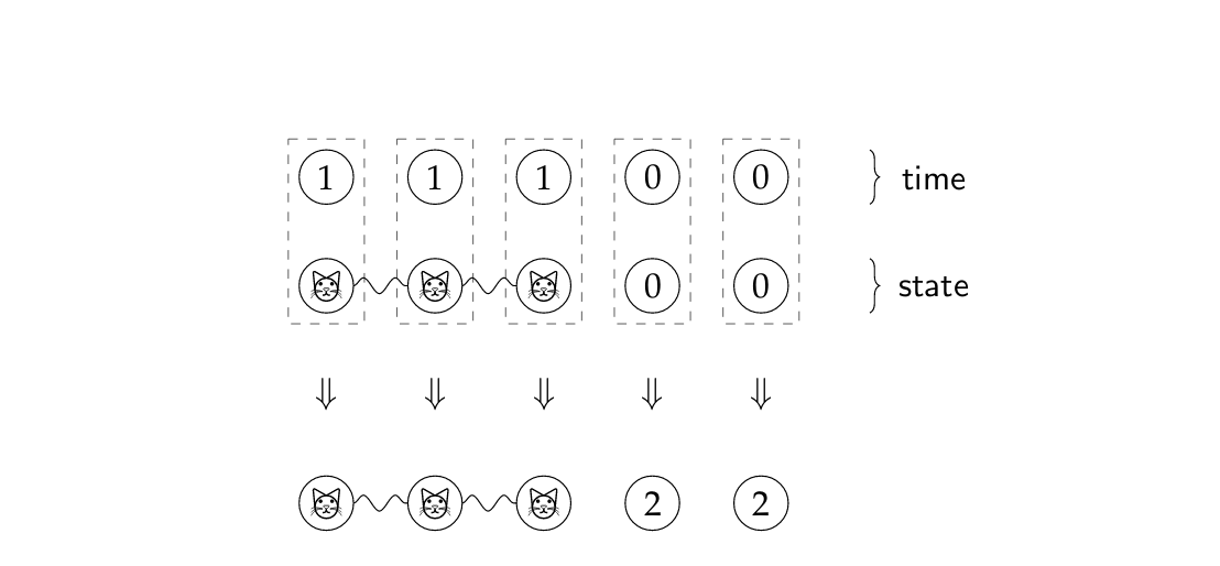
To see that we can have $\mathcal{H}$ act on particles of dimension $3$ (qutrits) rather than particles of dimension $4$ , note that the degree of freedom corresponding to $|\textsf{time}(t)\rangle \otimes |\textsf{state}(t)\rangle = |0\rangle \otimes |1\rangle$ is unused, as the $t^{\text{th}}$ qubit of the state is never nonzero until timestamp $t$ . Thus, we can take the vectors

$\begin{aligned} |0\rangle := |1\rangle\otimes|0\rangle, |1\rangle := |1\rangle\otimes|1\rangle, |2\rangle := |0\rangle\otimes|0\rangle \end{aligned}$

as a basis for each qutrit.

Even though we’ve shown that the clock Hamiltonian for our original circuit cannot be used to prove NLTS (which is still weaker than the original Quantum PCP conjecture) this does not necessarily rule out the use of this approach for other “hard” circuits which might then allow us to prove NLTS. Furthermore, NLETS is independently interesting, as the notion of being low “Hamming distance” away from vectors is exactly what is used in error-correcting codes.

References

[1] Sanjeev Arora and Boaz Barak. Computational complexity: a modern approach. Cambridge University Press, 2009.
[2] Chinmay Nirkhe, Umesh Vazirani, and Henry Yuen. Approximate low-weight check codes and circuit lower bounds for noisy ground states. arXiv preprint arXiv:1802.07419, 2018.
[3] Dorit Aharonov, Wim van Dam, Julia Kempe, Zeph Landau, Seth Lloyd, and Oded Regev. Adiabatic quantum computation is equivalent to standard quantum computation. SIAM J. Comput., 2007.

	James Cross on GPT as an “Intelligence…
	Thoughts on AI safet… on AI will change the world, but…
	Anonymous on An alarming trend in K-12 Math…
	Interview about this… on Men in Computer Science
	Interview about this… on The Swiss Army Knife of C…

Towards Quantum PCP: A Proof of the NLETS Theorem

Introduction

Progress

Reformulation: NLTS conjecture

Progress: NLETS theorem

Quantum circuits

Lightcones, effect zones, shadow zones

Toward the Feynman-Kitaev clock

Proof of NLETS

Back to NLTS – Tempering our Optimism

The Woes of Constant-Dimensional Lattices

Linearizing the Hamiltonian

References

Published by richardmwang

Leave a Reply Cancel reply

Introduction

Progress

Reformulation: NLTS conjecture

Progress: NLETS theorem

Quantum circuits

Lightcones, effect zones, shadow zones

Toward the Feynman-Kitaev clock

Proof of NLETS

Back to NLTS – Tempering our Optimism

The Woes of Constant-Dimensional Lattices

Linearizing the Hamiltonian

References

Share this:

Like this:

Related

Published by richardmwang

Leave a Reply Cancel reply