In this blog post, we give a broad overview of quantum walks and some quantum walks-based algorithms, including traversal of the glued trees graph, search, and element distinctness [3; 7; 1]. Quantum walks can be viewed as a model for quantum computation, providing an advantage over classical and other non-quantum walks based algorithms for certain applications.
Continuous time quantum walks
We begin our discussion of quantum walks by introducing the quantum analog of the continuous random walk. First, we review the behavior of the classical continuous random walk in order to develop the definition of the continuous quantum walk.
Take a graph with vertices and edges . The adjacency matrix of is defined as follows:
And the Laplacian is given by:
The Laplacian determines the behavior of the classical continuous random walk, which is described by a length vector of probabilities, p(t). The th entry of p(t) represents the probability of being at vertex at time . p(t) is given by the following differential equation:
which gives the solution .
Recalling the Schrödinger equation , one can see that by inserting a factor of on the left hand side of the equation for p(t) above, the Laplacian can be treated as a Hamiltonian. One can see that the Laplacian preserves the normalization of the state of the system. Then, the solution to the differential equation:
,
which is , determines the behavior of the quantum analog of the continuous random walk defined previously. A general quantum walk does not necessarily have to be defined by the Laplacian; it can be defined by any operator which “respects the structure of the graph,” that is, only allows transitions to between neighboring vertices in the graph or remain stationary [7]. To get a sense of how the behavior of the quantum walk differs from the classical one, we first discuss the example of the continuous time quantum walk on the line, before moving on to the discrete case.
Continuous time quantum walk on the line
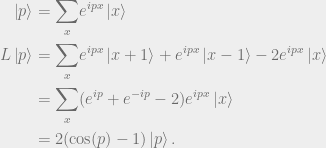
An important example of the continuous time quantum walk is that defined on the infinite line. The eigenstates of the Laplacian operator for the graph representing the infinite line are the momentum states with eigenvalues , for in range . This can be seen by representing the momentum states in terms of the position states and applying the Laplacian operator:
Hence the probability distribution at time , , with initial position is given by:
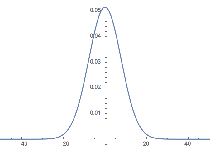
Figure 1.a) Probability distribution for continuous time quantum walk on the infinite line at time . Figure 1.b) Approximate probability distribution of the continuous time random walk on the infinite line at time .
While the probability distribution for the classical continuous time random walk on the same graph approaches, for large , , or a Gaussian of width . One can see that the quantum walk has its largest peaks at the extrema, with oscillations in between that decrease in amplitude as one approaches the starting position at . This is due to the destructive interference between states of different phases that does not occur in the classical case. The probability distribution of the classical walk, on the other hand, has no oscillations and instead a single peak centered at , which widens and flattens as increases.
Walk on the glued trees graph
A glued tree is a graph obtained by taking two binary trees of equal height and connecting each of the leaves of one of the trees to exactly two leaves of the other tree so that each node that was a leaf in one of the original trees now has degree exactly . An example of such a graph is shown in Figure 2.
Figure 2: An example of a glued tree graph, from [2].
The time for the quantum walk on this graph to reach the right root from the left one is exponentially faster than in the classical case. Consider the classical random walk on this graph. While in the left tree, the probability of transitioning to a node in the level one to the right is twice that of transitioning to a node in the level one to the left. However, while in the right tree, the opposite is true. Therefore, one can see that in the middle of the graph, the walk will get lost, as, locally, there is no way to determine which node is part of which tree. It will instead get stuck in the cycles of identical nodes and will have exponentially small probability of reaching the right node.
To construct a continuous time quantum walk on this graph, we consider the graph in terms of columns. One can visualize the columns of Figure 2 as consisting of all the nodes equidistant from the entrance and exit nodes. If each tree is height , then we label the columns , where column contains the nodes with shortest path of length from the leftmost root node. We describe the state of each column as a superposition of the states of each node in that column. The number of nodes in column , , will be for and for . Then, we can define the state as:
The factor of latex ensures that the state is normalized. Since the adjacency matrix of the glued tree is Hermitian, then we can treat as the Hamiltonian of the system determining the behavior of the quantum walk. By acting on this state with the adjacency matrix operator , we get the result (for ):
Then for , we get the same result, because of symmetry.
For :
The case of is symmetric. One can see that the walk on this graph is equivalent to the quantum walk on the finite line with nodes corresponding to the columns. All of the edges, excluding that between columns and , have weight . The edge between column and has weight .
The probability distribution of the quantum walk on this line can be roughly approximated using the infinite line. In the case of the infinite line, the probability distribution can be seen as a wave propagating with speed linear in the time . Thus, in time linear in , the probability that the state is measured at distance from the starting state is . In [3] it is shown that the fact that the line is finite and has a single differently weighted edge from the others (that between and ) does not change the fact that in polynomial time, the quantum walk will travel from the left root node to the right one, although in this case there is no limiting distribution as the peaks oscillate. This was the first result that gives an exponential speed up over the classical case using quantum walks.
Figure 3: Although the quantum walk on the glued trees graph does not have a limiting distribution, this is an example of the resulting probability distribution at time for a column glued tree graph. The x-axis corresponds to the columns. One can see that the probability of being at the columns at either extremes is significantly larger than that of being in the middle of the graph. In contrast, the classical random walk takes exponential time to ever reach the exit root node.
Discrete time quantum walks
In this section, we will first give an introduction to the discrete quantum walk, including the discrete quantum walk on the line and the Markov chain quantum walk, as defined in [7]. Next, we discuss how Grover search can be viewed as a quantum walk algorithm, which leads us into Ambainis’s quantum-walks based algorithm from [1] for the element distinctness problem, which gives a speed up over classical and other quantum non-walks based algorithms.
The discrete time quantum walk is defined by two operators: the coin flip operator, and the shift operator. The coin flip operator determines the direction of the walk, while the shift operator makes the transition to the new state conditioned on the result of the coin flip. The Hilbert space governing the walk is , where corresponds to the space associated with the result of the coin flip operator, and corresponds to the locations in the graph on which the walk is defined.
For example, consider the discrete time walk on the infinite line. Since there are two possible directions (left or right), then the Hilbert space associated with the coin flip operator is two dimensional. In the unbiased case, the coin flip is the Hadamard operator,
and shift operator that produces the transition from state to or , conditioned on the result of the coin flip, is .
Each step of the walk is determined by an application of the unitary operator . If the walk starts at position , then measuring the state after one application of gives with probability and with probability . This is exactly the same as the case of the classical random walk on the infinite line; the difference between the two walks becomes apparent after a few steps.
For example, the result of the walk starting at state after 4 steps gives:
One can see that the distribution is becoming increasingly skewed towards the right, while in the classical case the distribution will be symmetric around the starting position. This is due to the destructive interference discussed earlier. The distribution after time steps is shown in Figure 4.
Figure 4: Distribution at time , with on the x-axis corresponding to position .
Now, consider the walk starting at state :
This distribution given by this walk is the mirror image of the first. To generate a symmetric distribution, consider the start state . The resulting distribution after steps will be , where is the probability distribution after steps resulting from the start state and is the probability distribution after steps resulting from the start state . The result will be symmetric, with peaks near the extrema, as we saw in the continuous case.
Markov chain quantum walk
A reversible, ergodic Markov chain with states can be represented by a transition matrix with equal to the probability of transitioning from state to state and . Then, , where is an initial probability distribution over the states, gives the distribution after one step. Since for all , is stochastic and thus preserves normalization.
There are multiple ways to define a discrete quantum walk, depending on the properties of the transition matrix and the graph on which it is defined (overview provided in [4]). Here we look at the quantum walk on a Markov chain as given in [2]. For the quantum walk on this graph, we define state as the state that represents currently being at position and facing in the direction of . Then, we define the state as a superposition of the states associated with position :
The unitary operator,
,
acts as a coin flip for the walk on this graph. Since is reversible, we can let the shift operator be the unitary operator:
.
A quantum walk can also be defined for a non-reversible Markov chain using a pair of reflection operators (the coin flip operator is an example of a reflection operator). This corresponds to the construction given in [7].
Search as a quantum walk algorithm
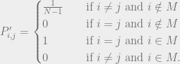
Given a black box function and a set of inputs with , say we want to find whether an input exists for which equals some output value. We refer to the set of inputs for which this is true as marked. Classically, this requires queries, for nonempty . Using the Grover search algorithm, this problem requires quantum queries. In this section, we give a quantum walks based algorithm that also solves this problem in time. If we define a doubly stochastic matrix with uniform transitions, then we can construct a new transition matrix from as:
Then, when the state of the first register is unmarked, the operator defined in the previous section acts as a diffusion over its neighbors. When the state in the first register is marked, then will act as the operator , and the walk stops, as a marked state has been reached. This requires two queries to the black box function: one to check whether the input is marked, and then another to uncompute. By rearranging the order of the columns in so that the columns corresponding to the non-marked elements come before the columns corresponding to the marked elements, we get:
where gives the transitions between non-marked elements and gives the transitions from non-marked to marked elements.
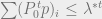
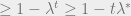
We now look at the hitting time of the classical random walk. Assume that there is zero probability of starting at a marked vertex. Then, we can write the starting distribution , where the last elements of , corresponding to the marked elements, are zero, as , where are the eigenvalues of , and are the corresponding eigenvectors, with the last entries zero. Let be the principal (largest) eigenvalue. Then, the probability that, after steps, a marked element has not yet been reached will be . Then, the probability that a marked element has been reached in that time will be . Setting gives probability that a marked element will be reached in that time.
The eigenvalues of will be and . Then, the classical hitting time will be:
It can be showed that for a walk defined by a Markov chain, the classical hitting time will be , where , the spectral gap, and [2].
Magniez et al proved in [6] that for a reversible, ergodic Markov chain, the quantum hitting time for a walk on this chain is within a factor of the square root of the classical hitting time. Since the walk on this input acts as a walk on a reversible Markov chain until a marked element is reached, then this is also true for a walk defined by our transition matrix . This arises from the fact that the spectral gap of the matrix describing the quantum walk corresponding to stochastic matrix is quadratically larger than the spectral gap of the matrix describing the classical random walk corresponding to , the proof of which is given in [2]. Thus, the quantum hitting time is , which exactly matches the quantum query complexity of Grover search.
Element distinctness problem
Now, we describe Ambainis’s algorithm given in [1] for solving the element distinctness problem in time, which produces a speed up over the classical algorithm, which requires queries, and also over other known quantum algorithms that do not make use of quantum walks, which require queries. The element distinctness problem is defined as follows: given a function on a size set of inputs
,…,,
determine whether there exists a pair for which . As in the search problem defined in the previous section, this is a decision problem; we are not concerned with finding the values of these pairs, only whether at least one exists.
The algorithm is similar to the search algorithm described in the previous section, except we define the walk on a Hamming graph. A Hamming graph is defined as follows: each vertex corresponds to an -tuple, (,…,), where for all and repetition is allowed (that is, may equal for ), and is a parameter we will choose. Edges will exist between vertices that differ in exactly one coordinate (order matters in this graph). We describe the state of each vertex as:
,…,,…,
Then, moving along each edge that replaces the th coordinate with such that requires two queries to the black box function to erase and compute . In the case, the marked vertices will be those that contain some for . Since the function values are stored in the description of the state, then no additional queries to the black box are required to check if in a marked state.
The transition matrix is given by . is the all one matrix, and the superscript denotes the operator acting on the th coordinate. The factor of normalizes the degree, since the graph is regular. We can compute the spectral gap of this graph to be (for details of this computation, see [2]). Then, noting that that the fraction of marked vertices, , is , classically, the query complexity is , where is the queries required to construct the initial state. Setting the parameters equal to minimize with respect to gives classical query complexity , as expected.
Then in the quantum case, queries are still required to set up the state. queries are required to perform the walk until a marked state is reached, by [6]. Setting parameters equal gives queries, as desired.
[1] Ambainis, A. Quantum walk algorithm for element distinctness, SIAM Journal on Computing 37(1):210-239 (2007). arXiv:quant-ph/0311001
[3] Childs, A., Farhi, E. Gutmann, S. An example of the difference between quantum and classical random walks. Journal of Quantum Information Processing, 1:35, 2002. Also quant-ph/0103020.
[4] Godsil, C., Hanmeng, Z. Discrete-Time Quantum Walks and Graph Structures (2018). arXiv:1701.04474
[5] Kempe, J. Quantum random walks: an introductory overview, Contemporary Physics, Vol. 44 (4) (2003) 307:327. arXiv:quant-ph/0303081
[6] Magniez, F., Nayak, A., Richter, P.C. et al. On the hitting times of quantum versus random walks, Algorithmica (2012) 63:91. https://doi.org/10.1007/s00453-011-9521-6


![[-\pi,\pi]](https://s0.wp.com/latex.php?latex=%5B-%5Cpi%2C%5Cpi%5D&bg=eeeeee&fg=666666&s=0&c=20201002)


 .
.
 .
.


![i \in [0,n]](https://s0.wp.com/latex.php?latex=i+%5Cin+%5B0%2Cn%5D&bg=eeeeee&fg=666666&s=0&c=20201002)

![i \in [n+1,2n+1]](https://s0.wp.com/latex.php?latex=i+%5Cin+%5Bn%2B1%2C2n%2B1%5D&bg=eeeeee&fg=666666&s=0&c=20201002)


![i \in [1,n-1]](https://s0.wp.com/latex.php?latex=i+%5Cin+%5B1%2Cn-1%5D&bg=eeeeee&fg=666666&s=0&c=20201002)

![i \in [n+2,2n]](https://s0.wp.com/latex.php?latex=i+%5Cin+%5Bn%2B2%2C2n%5D&bg=eeeeee&fg=666666&s=0&c=20201002)


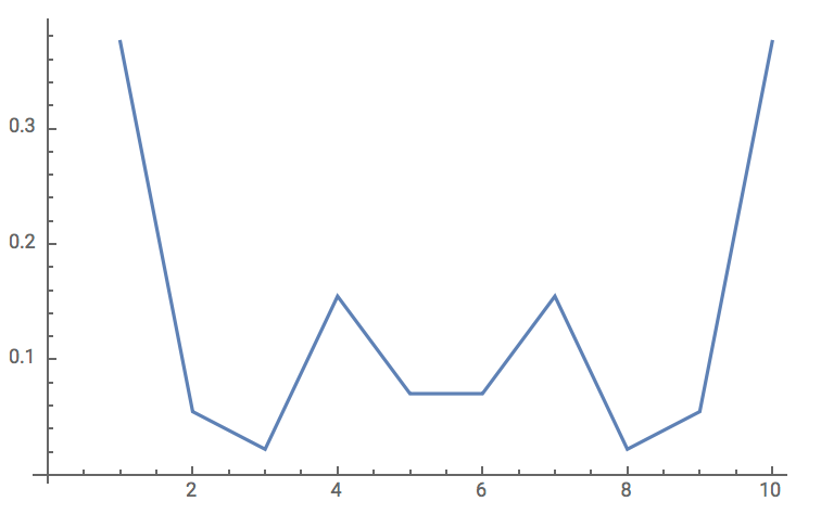
 column glued tree graph. The x-axis corresponds to the columns. One can see that the probability of being at the columns at either extremes is significantly larger than that of being in the middle of the graph. In contrast, the classical random walk takes exponential time to ever reach the exit root node.


 on the x-axis corresponding to position
  .
.


![P = \frac{1}{m(n-1)} \underset{i \in [1,m]}{\sum} (J - I)^{(i)}](https://s0.wp.com/latex.php?latex=P+%3D+%5Cfrac%7B1%7D%7Bm%28n-1%29%7D+%5Cunderset%7Bi+%5Cin+%5B1%2Cm%5D%7D%7B%5Csum%7D+%28J+-+I%29%5E%7B%28i%29%7D&bg=eeeeee&fg=666666&s=0&c=20201002)


Very nice post as are the other posts. Maybe it would be a good idea to leave a few days between consecutive postings.
Dear Dr. Nash, you may find related material in my book “Quantum Walks and Search Algorithms” (https://link.springer.com/book/10.1007/978-3-319-97813-0).