Nilin Abrahamsen nilin@mit.edu
Daniel Alabi alabid@g.harvard.edu
Mitali Bafna mitalibafna@g.harvard.edu
Emil Khabiboulline ekhabiboulline@g.harvard.edu
Juspreet Sandhu jus065@g.harvard.edu
Two-prover one-round (2P-1R) games have been the subject of intensive study in classical complexity theory and quantum information theory. In a 2P-1R game, a verifier sends questions privately to each of two collaborating provers , who then aim to respond with a compatible pair of answers without communicating with each other. Sharing quantum entanglement allows the provers to improve their strategy without any communication, illustrating an apparent paradox of the quantum postulates. These notes aim to give an introduction to the role of entanglement in nonlocal games, as they are called in the quantum literature. We see how nonlocal games have rich connections within computer science and quantum physics, giving rise to theorems ranging from hardness of approximation to the resource theory of entanglement.
Introduction
In these notes we discuss 2-prover 1-round games and the classical complexity of approximating the value of such games in the setting where the provers can share entanglement. That is, given the description of a game, we ask how hard it is to estimate the winning probability of the best winning strategy of the entangled provers. Let us first formally define games and its relation to the label cover problem. We write![{ [n]=\{1,\ldots,n\}}](https://s0.wp.com/latex.php?latex=%7B+%5Bn%5D%3D%5C%7B1%2C%5Cldots%2Cn%5C%7D%7D&bg=eeeeee&fg=000000&s=0&c=20201002) .
.
Definition (Label cover)
A label cover instance consists of variable sets
 ![{ S=\{s_i\}_{i\in[n]},T=\{t_j\}_{j\in[n]}}](https://s0.wp.com/latex.php?latex=%7B+S%3D%5C%7Bs_i%5C%7D_%7Bi%5Cin%5Bn%5D%7D%2CT%3D%5C%7Bt_j%5C%7D_%7Bj%5Cin%5Bn%5D%7D%7D&bg=eeeeee&fg=000000&s=0&c=20201002) , alphabet set
, alphabet set  , and a collection
  of constraints of the form
  . Given an assignment (or coloring)
  we define its value to be
  . Define the value of
  to be the maximum over all possible assignments, i.e.
  .
Many familiar computational problems can be formulated as a label cover, such as
.
Many familiar computational problems can be formulated as a label cover, such as  ,
,  , and
, and  .
.

Definition (2-prover 1-round game)
Let be a label cover instance. We can then associate the following two-prover one-round game
  with . Let
  be two provers who cannot communicate, and let
  be the verifier. Given the label cover instance , the verifier uniformly samples a constraint
  and sends
  to
to  and
and  to
to  . The provers then reply with
  and
and  respectively to . Finally, outputs
  if and only if
  .
.
 with probability
  . That is, the value of the game equals that of the label cover instance. However, this is with the assumption that provers can only use deterministic strategies or convex combinations of these (that is, using shared randomness). If the provers share an entangled quantum state, then the provers (who still cannot communicate) can enjoy correlations that allow them to win with a higher probability than classically. In the quantum literature, these 2P-1R games are known as nonlocal games referring to the fact that the correlations arise without signaling between the provers. We are concerned with the complexity of approximating the winning probability of this strategy.
We refer to the optimal winning probability within some class (classical or entangled) of strategies as the classical and quantum value of the game, respectively, and we use the terms quantum strategy and entangled strategy interchangeably.
Fixing different constraint families in the label cover game changes the complexity of finding the (classical and entangled) values of the game. We will show that approximating the entangled value of XOR games, or more generally unique games (to be defined later on), is possible in polynomial time. This is remarkable because a famous conjecture known as the unique games conjecture says that approximating the classical value of unique games is NP-hard. In contrast, we will see that for unrestricted edge constraints, it is NP-hard to approximate the entangled value of a nonlocal game. Thus, hardness of approximation of the game’s value, established by the celebrated PCP theorem , still applies in the presence of entanglement. In the quantum world, we have new complexity classes such as QMA (which can be regarded as “quantum NP”), so one may conjecture whether approximating the entangled value of a general game is QMA-hard (the games formulation of the quantum PCP conjecture ). We will indicate progress in this direction but will explicitly demonstrate the NP-hardness result.
Entanglement is often regarded as an expensive resource in quantum information because it is difficult to produce and maintain. Hence, even if sharing entanglement can improve the success probability of winning a game, the resource consumption may be costly. We will conclude by discussing lower bounds on the number of shared entangled bits required to achieve the optimal value of a game.
. That is, the value of the game equals that of the label cover instance. However, this is with the assumption that provers can only use deterministic strategies or convex combinations of these (that is, using shared randomness). If the provers share an entangled quantum state, then the provers (who still cannot communicate) can enjoy correlations that allow them to win with a higher probability than classically. In the quantum literature, these 2P-1R games are known as nonlocal games referring to the fact that the correlations arise without signaling between the provers. We are concerned with the complexity of approximating the winning probability of this strategy.
We refer to the optimal winning probability within some class (classical or entangled) of strategies as the classical and quantum value of the game, respectively, and we use the terms quantum strategy and entangled strategy interchangeably.
Fixing different constraint families in the label cover game changes the complexity of finding the (classical and entangled) values of the game. We will show that approximating the entangled value of XOR games, or more generally unique games (to be defined later on), is possible in polynomial time. This is remarkable because a famous conjecture known as the unique games conjecture says that approximating the classical value of unique games is NP-hard. In contrast, we will see that for unrestricted edge constraints, it is NP-hard to approximate the entangled value of a nonlocal game. Thus, hardness of approximation of the game’s value, established by the celebrated PCP theorem , still applies in the presence of entanglement. In the quantum world, we have new complexity classes such as QMA (which can be regarded as “quantum NP”), so one may conjecture whether approximating the entangled value of a general game is QMA-hard (the games formulation of the quantum PCP conjecture ). We will indicate progress in this direction but will explicitly demonstrate the NP-hardness result.
Entanglement is often regarded as an expensive resource in quantum information because it is difficult to produce and maintain. Hence, even if sharing entanglement can improve the success probability of winning a game, the resource consumption may be costly. We will conclude by discussing lower bounds on the number of shared entangled bits required to achieve the optimal value of a game.
Notation and quantum postulates
Let us first establish notation and define what is meant by an entangled strategy. In keeping with physics notation we write a column vector as and its conjugate-transpose (a row vector) as
  . More generally the conjugate-transpose (Hermitian conjugate) of a matrix
  is written
  . Then
  is the inner product of two vectors (a scalar) and
  the outer product (a rank-1 matrix). A matrix is said to be Hermitian if
  . A matrix is positive semidefinite , written
  , if
, if  for some matrix
  . We write the identity matrix as
  , denote by
  the set of
  -by- Hermitian matrices.
Observables, states, and entanglement
In a quantum theory the observables are Hermitian operators on a vector space
  . It then makes sense to say that a state is a functional
  on the set of observables. That is, to specify the state of a physical system means giving a (expected) value for each observable. It turns out states are linear functionals of the observables, and such functionals can be written
  for some -by- matrix
  . We call the density matrix and require moreover that is positive semidefinite and has trace . Every density matrix is a convex combination of rank-one projections
  known as pure states. The unit vectors
  are also themselves known as pure states.
If the state of one particle is described by a vector in (referring here to pure states), then two particles are described by a vector in the tensor product
are also themselves known as pure states.
If the state of one particle is described by a vector in (referring here to pure states), then two particles are described by a vector in the tensor product  . The two particles are entangled if their state is not in the form of a pure tensor
  . We also write product states as
  , omitting the tensor symbol.
Quantum measurements
A quantum measurement can be described in terms of a projection-valued measure (PVM). Definition 1 (PVM) A projection-valued measure on vector space (where the quantum states live) is a list of projection matrices  on such that
  for
for  and
and  . The PVM describes a measurement which, on state outputs measurement outcome
  with probability
  . The quantum state after obtaining outcome is
  .
When the projections are rank-one projections
.
When the projections are rank-one projections  we say that we measure in the basis
  . In this case the probability of outcome in state
  is
is  , and the post-measurement state is simply
  .
Applying the measurement
.
Applying the measurement  on the left half of a two-particle state
  means applying the PVM
  on the two-particle state.
Quantum strategies for nonlocal games
We now introduce the notion of a quantum strategy for a nonlocal game. Each prover holds a particle, say with state space, and Alices particle may be entangled with Bob’s. The global state is  . Each player receives a question from the verifier and then chooses a measurement (a PVM) depending on the question. The player applies the measurement to their own particle and responds to the verifier with their measurement outcome. Hence for Alice we specify
  PVM’s
PVM’s  where
where  is a question, and each PVM is a list
  . By definition 1, given questions
  the probability that Alice outputs
  and Bob outputs
  is
is

Quantum strategies beat classical ones
For any 2P-1R game , let
, let  be the maximum probability — over the players’ classical strategies — that the verifier accepts and
  the maximum probability that the verifier accepts when the provers use qubits such that player 1’s qubits are entangled with those of player 2.
The game of Clauser, Horne, Shimony, and Holt (CHSH) has the property that the provers can increase their chance of winning by sharing an entangled pair of qubits, even when no messages are exchanged between the players. We show that there’s a characterization of the CHSH game’s value
the maximum probability that the verifier accepts when the provers use qubits such that player 1’s qubits are entangled with those of player 2.
The game of Clauser, Horne, Shimony, and Holt (CHSH) has the property that the provers can increase their chance of winning by sharing an entangled pair of qubits, even when no messages are exchanged between the players. We show that there’s a characterization of the CHSH game’s value  which is better than the classical value
  . Let us first define XOR games, of which the CHSH game is a special case.
Definition (XOR game)
An XOR game is a 2-player classical game (the questions and answers are classical bits) where:- Questions
are asked according to some distribution
- Answers
are provided by players (call them Alice and Bob).
- The verifier computes a predicate
used to decide acceptance/rejection.
Definition (CHSH Game)
An XOR game with where
where  are independent random bits and
  .
To win the CHSH game, Alice and Bob need to output bits (from Alice) and (from Bob) that disagree if
.
To win the CHSH game, Alice and Bob need to output bits (from Alice) and (from Bob) that disagree if  and agree otherwise.
If Alice and Bob are classical then they can do no better than by always outputting
and agree otherwise.
If Alice and Bob are classical then they can do no better than by always outputting  , say, in which case they win in the three out of four cases when one of the questions is . Equivalently,
  where is the CHSH game. This is the content of Bell’s inequality :
Lemma (Bell’s Inequality)
For any two functions , we have
![{ {\mathop{\mathbb{P}}}_{x, y\in\{0, 1\}}\left[g(x)\oplus h(y) = x\wedge y\right] \leq \frac{3}{4} }](https://s0.wp.com/latex.php?latex=%7B+%7B%5Cmathop%7B%5Cmathbb%7BP%7D%7D%7D_%7Bx%2C+y%5Cin%5C%7B0%2C+1%5C%7D%7D%5Cleft%5Bg%28x%29%5Coplus+h%28y%29+%3D+x%5Cwedge+y%5Cright%5D+%5Cleq+%5Cfrac%7B3%7D%7B4%7D+%7D&bg=eeeeee&fg=000000&s=0&c=20201002) where
where  and
and  are independent uniformly random bits.
Proof. The probability of any event is a multiple of
 so it suffices to show that
 ![{ {\mathop{\mathbb{P}}}_{x, y\in\{0, 1\}}\left[g(x)\oplus h(y) = x\wedge y\right]\neq1}](https://s0.wp.com/latex.php?latex=%7B+%7B%5Cmathop%7B%5Cmathbb%7BP%7D%7D%7D_%7Bx%2C+y%5Cin%5C%7B0%2C+1%5C%7D%7D%5Cleft%5Bg%28x%29%5Coplus+h%28y%29+%3D+x%5Cwedge+y%5Cright%5D%5Cneq1%7D&bg=eeeeee&fg=000000&s=0&c=20201002) . So assume for contradiction that
. So assume for contradiction that  for all pairs
  . Then we have that
  and
and  which implies that
  . But then
  which is a contraction.
The strategy
The entangled strategy for the CHSH game requires that Alice and Bob each hold a qubit, so that their two qubits together are described by a vector in . The two qubits together are in the state
 forming what is known as an EPR (Einstein-Podolsky-Rosen) pair. Now for
 ![{ \theta\in[-\pi, \pi]}](https://s0.wp.com/latex.php?latex=%7B+%5Ctheta%5Cin%5B-%5Cpi%2C+%5Cpi%5D%7D&bg=eeeeee&fg=000000&s=0&c=20201002) define
define  and
and  .
Now we describe a (quantum) strategy with winning probability
.
Now we describe a (quantum) strategy with winning probability  . In each case Alice and Bob respond with their measurement outcome, where subscripts of the measurement basis vectors correspond to the answer to be sent back to the verifier.
- If
, Alice measures in basis
. If
, Alice measures in
. Alice answers bit
if outcome is
and answers
otherwise.
- If
, Bob measures in basis
. If
, Bob measures in
.
- Each player responds with their respective measurement outcome.
.
Proof. We will show that for each pair of questions
the pair of answers  is correct with probability
  . We can split the pairs of questions into the two cases
  and
and  :
:
- (
are all analogous: in each case Alice an Bob must output the same answer, and in each case Bob’s measurement basis is almost the same as Alice’s except rotated by a small angle
. Of the three above cases we consider the one where
and check that indeed the two measurement outcomes agree with probability
collapses to
. Indeed, since the question was
. This means that Alice applies the measurement
on the global state. The post-measurement state is the normalization of
because
can be viewed as a Kronecker delta of
. In particular, Bob is now in the pure state
. Because Bob received question
Therefore his probability of correctly outputting
is
- (
where Alice and Bob are supposed to give different answers. Alice measures in basis consisting of
and
. If Alice gets outcome
. Therefore when Bob applies the measurement in basis
he mistakenly outputs
.
![{ {\mathop{\mathbb{P}}}[\text{Bob gets outcome }a] = |\langle\beta_a(\tfrac{\pi}{8}) |{a}\rangle |^2 = \cos^2\left(\frac{\pi}{8}\right) }](https://s0.wp.com/latex.php?latex=%7B+%7B%5Cmathop%7B%5Cmathbb%7BP%7D%7D%7D%5B%5Ctext%7BBob+gets+outcome+%7Da%5D+%3D+%7C%5Clangle%5Cbeta_a%28%5Ctfrac%7B%5Cpi%7D%7B8%7D%29+%7C%7Ba%7D%5Crangle+%7C%5E2+%3D+%5Ccos%5E2%5Cleft%28%5Cfrac%7B%5Cpi%7D%7B8%7D%5Cright%29+%7D&bg=eeeeee&fg=000000&s=0&c=20201002)
Corollary
It turns out that this lower bound is sharp, that is, the strategy just described is optimal.
Lemma
The value of the CHSH game using a quantum strategy is at most .
Proof.
We can describe the quantum strategy of Alice and Bob in an XOR game by (i) a shared quantum state
.
Proof.
We can describe the quantum strategy of Alice and Bob in an XOR game by (i) a shared quantum state  (note that for the CHSH game,
  ); (ii) measurements
  for every question
  sent to Alice; (iii) measurements
  for every question
  sent to Bob.
The probability of answering
sent to Bob.
The probability of answering  given questions
  is
is  . Now let us write
  and
and  so that for any , we can write
 Note that since the possible outcomes here are finite,
  are Hermitian and we may assume have bounded norm of 1. Furthermore, we assume that are observables so that
  .
Now denoting
.
Now denoting  as the XOR predicate to be computed, we can write the quantum game value as
 where the summation
  has been evaluated in the last line.
Now note that the first term is independent of the quantum strategy and as a result equals the value of the uniformly random strategy which is 1/2. So we proceed to focus on the second term. Note that for CHSH
has been evaluated in the last line.
Now note that the first term is independent of the quantum strategy and as a result equals the value of the uniformly random strategy which is 1/2. So we proceed to focus on the second term. Note that for CHSH  simplifying the second term to
 Next, we invoke Tsirelson’s Theorem (See Theorem 3) to bound this second term as
 where we have used Cauchy-Schwartz and the concavity of the
  function.
This completes our proof showing the exact characterization of the value (
function.
This completes our proof showing the exact characterization of the value ( ) of the CHSH game using a quantum strategy. This proof is an adaptation of the one in [12].
 matrix
  , the following are equivalent:
- There exist
such that for any
. Further this would imply that
;
- There exist real unit vectors
for
such that
;
![{ s, t\in[n]}](https://s0.wp.com/latex.php?latex=%7B+s%2C+t%5Cin%5Bn%5D%7D&bg=eeeeee&fg=000000&s=0&c=20201002)
Entangled unique games are easy
The CHSH game provides the first example that the entangled value of a nonlocal game can exceed the classical value . XOR-games like the CHSH game are the special case corresponding to alphabet size  of the class of unique games :
Definition (Unique Games)
A 2-prover 1-round game is called a unique game if its constraints are of the form where
where  is a permutation of the alphabet for each edge
  .
The famous unique games conjecture (UGC) by Khot says that is NP-hard to approximate for unique games. Surprisingly, Kempe et al. showed that a natural semidefinite relaxation for unique games yields an approximation to the entangled value which can be computed in polynomial time. In other words the UGC is false for entangled provers, in contrast to the classical case where the conjecture is open.
.
The famous unique games conjecture (UGC) by Khot says that is NP-hard to approximate for unique games. Surprisingly, Kempe et al. showed that a natural semidefinite relaxation for unique games yields an approximation to the entangled value which can be computed in polynomial time. In other words the UGC is false for entangled provers, in contrast to the classical case where the conjecture is open.
Theorem 4 There is an efficient (classical) algorithm which takes a description of a nonlocal game
as its input and outputs  such that
 Put differently, if
  and
and  , then
![{ \varepsilon^*\in[\hat\varepsilon,6\hat\varepsilon] }](https://s0.wp.com/latex.php?latex=%7B+%5Cvarepsilon%5E%2A%5Cin%5B%5Chat%5Cvarepsilon%2C6%5Chat%5Cvarepsilon%5D+%7D&bg=eeeeee&fg=000000&s=0&c=20201002)
The algorithm of theorem 4 proceeds by relaxing the set of quantum strategies to a larger convex set
 of pseudo-strategies and maximizing over instead of actual strategies, a much easier task. In approximation theory one often encounters a collection of hypothetical moments not arising from a distribution, known as a pseudo-distribution. In contrast, our pseudo-strategies are actual conditional probability distributions on answers (conditional on the questions). What makes a set of “pseudo”-strategies rather than actual strategies is that they may enjoy correlations which cannot be achieved without communication.
Convex relaxation of quantum strategies
We will define to be a class of conditional probability distributions  on answers given questions. We will require that the pseudo-strategies satisfy a positive semidefinite constraint when arranged in matrix form. In particular this matrix has to be symmetric, so we symmetrize the conditional probability by allowing each of and to be either a question for Alice or for Bob. That is, we extend the domain of definition for from
  to
to  where
where  and
and  are the question sets. So each question and and answer and can be either for Alice or Bob — we indicate this by changing notation from
  to
to  and for the answers replacing by
  .
.
Definition 5 (Block-matrix form) Given a function
 defined on
  with
with  and
and  , define a
  -by- matrix
  whose rows are indexed by pairs
  and columns by pairs
  , and whose entries are
 In other words consists of
  -by- blocks where the block
  at position
  contains the entries
  .
. Definition 5 is simply a convenient change of notation and we identify
 with , using either notation depending on the context.
Definition 6 (Pseudo-strategies) Let
and be the question sets for Alice and Bob, respectively. We say that ![{ \tilde{P}=\tilde{P}(\cdot\cdot|\cdot\cdot):\Sigma^2\times (S\cup T)^2\rightarrow[0,1]}](https://s0.wp.com/latex.php?latex=%7B+%5Ctilde%7BP%7D%3D%5Ctilde%7BP%7D%28%5Ccdot%5Ccdot%7C%5Ccdot%5Ccdot%29%3A%5CSigma%5E2%5Ctimes+%28S%5Ccup+T%29%5E2%5Crightarrow%5B0%2C1%5D%7D&bg=eeeeee&fg=000000&s=0&c=20201002) (or its matrix form ) is a pseudo-strategy if:
(or its matrix form ) is a pseudo-strategy if:
-
- For any pair of questions
.
- The blocks
 The algorithm outputs the maximum winning probability:
 over pseudo-strategies
  . This maximum is efficiently computable using standard semidefinite programming algorithms. As we will see, actual quantum strategies are in which immediately implies
  . It then remains to show that the optimal pseudo-strategy can be approximated by an actual entangled strategy, thus bounding the gap from to .
Quantum strategies are in
Let us establish that is indeed a relaxation of the class of quantum strategies, that is, it contains the quantum strategies. So suppose we are given a quantum strategy. By equation 1 the probability of answers and given questions and is of the form
 for some PVM’s and
  and some
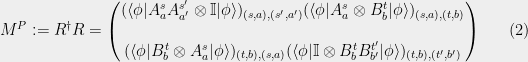
  . This conditional probability distibution is not immediately in the form of a pseudo-strategy because we cannot evaluate it on pairs of Alice-questions or pairs of Bob-questions. We therefore have to extend it, as follows: Place all the column vectors
  ,
,  side by side, and then append the vectors
  , resulting in a
  -by- matrix
  . We then define
 ![{ {P}(\cdot\cdot|\cdot\cdot):\Sigma^2\times(S\cup T)^2\rightarrow[0,1]}](https://s0.wp.com/latex.php?latex=%7B+%7BP%7D%28%5Ccdot%5Ccdot%7C%5Ccdot%5Ccdot%29%3A%5CSigma%5E2%5Ctimes%28S%5Ccup+T%29%5E2%5Crightarrow%5B0%2C1%5D%7D&bg=eeeeee&fg=000000&s=0&c=20201002) through its matrix form (see the comment below definition 5):
through its matrix form (see the comment below definition 5):
 defined in 2 is a pseudo-strategy, that is,
  .
.
Proof. We verify the conditions in definition 6. Condition 1 (
 ) holds because it is of the form
  . Condition 2 (Each block
  sums to ) holds because PVM’s sum to the identity. Condition 3 (Diagonal blocks
  are diagonal) holds because the projections in the PVM
  are mutually orthogonal, hence
  if
if  .
.
 is an (efficiently computable) upper bound for :
Corollary
 .
.
To finish the proof of theorem 4 we need to show that any pseudo-strategy
can be rounded to an actual quantum strategy with answer probabilities  such that

 or
or  , which will finish the proof of theorem 4.
Proof.[Proof of theorem 4] Let
 be a pseudo-strategy. We construct a quantum strategy approximating . Since is positive semidefinite we can write
 for some matrix
  and
and  . Now let us define vectors
  and
and  in
in  , and let
  and
and  be the same vectors normalized. The strategy is constructed as follows. Alice and Bob share the maximally entangled state
 Before deciding on Alice and Bob’s PVM’s and let us see what this choice of shared state means for the conditional distribution on answers (see equation (1)).

 is the entrywise dot product of matrices, and
  the entrywise complex inner product (Hilbert-Schmidt inner product).
We now choose the measurements. Given question , Alice measures in the PVM
the entrywise complex inner product (Hilbert-Schmidt inner product).
We now choose the measurements. Given question , Alice measures in the PVM  with
with
 Similarly, Bob on question applies the PVM with
 The condition 3 in definition 6 ensures that for any question , the vectors
  are orthogonal so that this is a valid PVM.
The measurement outcome “
are orthogonal so that this is a valid PVM.
The measurement outcome “ ” is interpreted as “fail”, and upon getting this outcome the player attempts the measurement again on their share of a fresh copy of
  . This means that the strategy requires many copies of the entangled state to be shared before the game starts. It also leads to the complication of ensuring that with high probability the players measure the same number of times before outputting their measurement, so that the outputs come from measuring the same entangled state.
By (*), at a given round of measurements the conditional distribution of answers is given by
. This means that the strategy requires many copies of the entangled state to be shared before the game starts. It also leads to the complication of ensuring that with high probability the players measure the same number of times before outputting their measurement, so that the outputs come from measuring the same entangled state.
By (*), at a given round of measurements the conditional distribution of answers is given by
 We wish to relate the LHS to
  , so to handle the factor
  each prover performs repeated measurements, each time on a fresh copy of , until getting an outcome
  . Moreover, to handle the factor
  , each prover consults public randomness and accepts the answer
 ![{ a\in[k]}](https://s0.wp.com/latex.php?latex=%7B+a%5Cin%5Bk%5D%7D&bg=eeeeee&fg=000000&s=0&c=20201002) with probability
with probability  and
and  respectively, or rejects and start over depending on the public randomness. Under a few simplifying conditions (more precisely, assuming that the game is uniform meaning that an optimal strategy exists where the marginal distribution on each prover’s answers is uniform), we can let
  for all
  , and one can ensure that the conditional probabilities of the final answers satisfy


General games are hard
We just saw that a specific class of games becomes easy in the presence of shared entanglement, in that semidefinite programming allows the entangled value to be approximated to within exponential precision in polynomial time. Does this phenomenon hold more generally, so that the value of entangled games can always be efficiently approximated? We answer in the negative, by constructing a game where is NP-hard to approximate to within inverse-polynomial factors. The complexity for 2P-1R entangled games can be strengthened to constant-factor NP-hardness, putting it on par with the classical PCP theorem. This result is used to prove (with some conditions) the games formulation of the quantum PCP theorem, which states that the entangled value of general games is QMA-hard to approximate within a constant factor.
Formulation of game
Given any instance of a -CSP (constraint satisfaction problem, where is the number of literals), we can define a clause-vs-variable game
  (see clause-vs-variable figure):
- The referee (verifier) randomly sends a clause to Alice (first prover) and a variable to Bob (second prover).
- Alice and Bob reply with assignments.
- The referee accepts if Alice’s assignment satisfies the clause and Bob’s answer is consistent with Alice’s.

 , given -CSP
  on variables
  , (1) the referee R randomly sends a clause
  to Alice A and a literal index
 ![{ t\in[k]}](https://s0.wp.com/latex.php?latex=%7B+t%5Cin%5Bk%5D%7D&bg=eeeeee&fg=000000&s=0&c=20201002) to Bob B, (2) A replies with an assignment
to Bob B, (2) A replies with an assignment  and B replies with assignment , (3) R accepts iff satisfies and
  . In variation (a), R sends an additional dummy index
 ![{ l\in[k]}](https://s0.wp.com/latex.php?latex=%7B+l%5Cin%5Bk%5D%7D&bg=eeeeee&fg=000000&s=0&c=20201002) , so that B replies with an additional assignment
, so that B replies with an additional assignment  , but he does not know which is the right variable. Equivalently, in (b) a third player Charlie C is introduced, but is played with two randomly chosen players. Since only parties can be maximally entangled and the players do not know who is playing the game, they cannot coordinate perfectly.
 NP-hardness of approximating the entangled value
To prove hardness, we rely on several results from classical complexity theory.Theorem 8 ([6]) Given an instance of 1-in-3 3SAT (a CSP), it is NP-hard to distinguish whether it is satisfiable or no assignments satisfy more than a constant fraction of clauses.
Theorem 9 ([2]) For a PCP game
 (emulating the CSP) and its oracularization
  (transformation to a 2P-1R game),
 and
and  is NP-hard for some -CSP. Here,
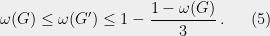
  denotes the maximum fraction of clauses that are simultaneously satisfiable. Theorem 9 relates the general game obtained from the CSP to a two-player one-round game
  , in terms of the value (probability of winning) the game. The first inequality, equivalently saying
  , is achieved since the players can answer the questions in the game to satisfy the clauses in . These theorems together imply that
  is NP-hard to approximate to within constant factors.
Allowing the two players to share entanglement can increase the game value to
is NP-hard to approximate to within constant factors.
Allowing the two players to share entanglement can increase the game value to  . Classical results do not necessarily carry over, but exploiting monogamy of entanglement allows us to limit the power of entangled strategies. One can show the following lemma, which is weaker than what we have classically.
Lemma 10 ([3]) There exists a constant
 such that for a CSP
  ,
,

 is the number of variables.
Combining Theorem 9 and Lemma 10, we have
is the number of variables.
Combining Theorem 9 and Lemma 10, we have
 Using Theorem 8, approximating
  is NP-hard to within inverse polynomial factors. Proving Lemma 10 takes some work in keeping track of approximations. For simplicity, we will show a less quantitative statement and indicate where the approximations come in.
Proposition 11 (adapted from [13])
is satisfiable iff  .
.
Proof of Proposition 11
The forward direction is straightforward: If is satisfiable, then there exists a perfect winning strategy where the questions are answered according to the satisfying assignment.
For the reverse direction, suppose there exists a strategy that succeeds with probability 1, specified by a shared entangled state  and measurements
  for Alice and
  for Bob, where the questions
 ![{ j\in[m]}](https://s0.wp.com/latex.php?latex=%7B+j%5Cin%5Bm%5D%7D&bg=eeeeee&fg=000000&s=0&c=20201002) ,
, ![{ t,l\in[k]}](https://s0.wp.com/latex.php?latex=%7B+t%2Cl%5Cin%5Bk%5D%7D&bg=eeeeee&fg=000000&s=0&c=20201002) and the answers are from the CSP’s alphabet. Since one of the questions/answers for Bob corresponds to a dummy variable that is irrelevant to the game, trace over the dummy variable to define a new measurement operator
and the answers are from the CSP’s alphabet. Since one of the questions/answers for Bob corresponds to a dummy variable that is irrelevant to the game, trace over the dummy variable to define a new measurement operator  . We can introduce a distribution on assignments to the relevant variables,

 on variables
  in any clause
  is
is
 has a satisfying assignment. To transform Eq. 7 to Eq. 8, we need a relation between the
  and
and  measurement operators and a way to commute the operators.
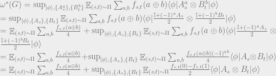
The success probability of the players’ strategy is expressed as
measurement operators and a way to commute the operators.
The success probability of the players’ strategy is expressed as
![{ P=\frac{1}{m}\sum_{j\in[m]}\frac{1}{k}\sum_{i\in C_j} \sum_{(a_1,\ldots,a_k)\vdash C_j} \langle{\psi}| A^j_{a_1,\ldots,a_k}\otimes \tilde{B}^i_{a_i} |{\psi}\rangle \,, }](https://s0.wp.com/latex.php?latex=%7B+P%3D%5Cfrac%7B1%7D%7Bm%7D%5Csum_%7Bj%5Cin%5Bm%5D%7D%5Cfrac%7B1%7D%7Bk%7D%5Csum_%7Bi%5Cin+C_j%7D+%5Csum_%7B%28a_1%2C%5Cldots%2Ca_k%29%5Cvdash+C_j%7D+%5Clangle%7B%5Cpsi%7D%7C+A%5Ej_%7Ba_1%2C%5Cldots%2Ca_k%7D%5Cotimes+%5Ctilde%7BB%7D%5Ei_%7Ba_i%7D+%7C%7B%5Cpsi%7D%5Crangle+%5C%2C%2C+%7D&bg=eeeeee&fg=000000&s=0&c=20201002) where is the index of one of the variables on which acts, and
where is the index of one of the variables on which acts, and  indicates that the assignment satisfies the clause. By positivity and summation to identity of the measurement operators and
  , each term is at most 1; for our hypothesis
  , each has to be 1. Hence, using orthogonality of the vectors
  for different
  , we have
 and
and  .
We now demonstrate that two different
.
We now demonstrate that two different  ,
,  commute, so that Bob can match any satisfied clause/variable.
 In the second line, we used (9) to relate the measurements. The third line follows by the orthogonality of
  for different
  . For the fourth equation, we simply swap
  since the questions are indistinguishable to Bob. Thus, we can see how the dummy variable comes into play. If we had assumed
  and kept track of approximations, we would find

 factors.
Now we are ready to transform Eq. 7 to Eq. 8 to conclude the proof.
factors.
Now we are ready to transform Eq. 7 to Eq. 8 to conclude the proof.
 In the second line, we used (10) to commute the measurement operators, along with their properties of orthogonality and summation to identity. For the third equality, we used (9) to relate Bob’s measurements to Alice’s, along with orthogonality of
  for different
  .
.
Constant-factor NP-hardness
The weakness in the above two-player game carries over from the original three-player variant. Thus, to achieve constant-factor NP-hardness of approximation, we could start with a different multiplayer game. Vidick [11] establishes the soundness of the “plane-vs-point” low-degree test (checking that the restriction of a low-degree polynomial to a plane matches its value at some point) in the presence of shared entanglement. Soundness , in the eponymous probabilistically checkable proof (PCP) formulation of the PCP theorem, refers to the verifier accepting a wrong proof with some bounded probability; bounding with a constant maps to constant-factor hardness of approximation. Here, soundness comes from a strong bound on error accumulation, similar to our approximate commutativity, but relies on the players’ Hilbert space being decomposable into three parts (i.e., there being three players). The particular game is constructed by combining the low-degree test with the 3-SAT test (encoding satisfying assignments in a low-degree polynomial), which can be reduced to the three-player QUADEQ test (testing satisfiability of a system of quadratic equations in binary variables, which is NP-complete). By the strong soundness result, the entangled value is NP-hard to approximate to within constant factors. Natarajan et al. [7] show that soundness holds even for two players, using a semidefinite program. They then construct a two-player game in a way similar to what we demonstrated.Constant-factor QMA-hardness
The above can be thought of as the games formulation of the classical PCP theorem holding under shared entanglement. A true quantum PCP theorem states that the entangled value of general games is QMA-hard to approximate to within constant factors. Natarajan et al. [8] establish such a theorem, but under randomized reductions. This requirement stems from the lack of a sufficiently strong QMA-hardness result for local Hamiltonians (the quantum analog of CSPs). The soundness of the two-player low-degree test above is one instrumental component in the proof.How much entanglement is needed?
We now focus on the question of quantifying exactly how much entanglement is needed to play XOR games optimally. As we shall see, the answer depends on the size of the question sets posed to Alice & Bob in the game. The previous bound given by Tsirelson [10] (see table below) is tight for certain families of games, but is not tight for other families of games (such as a generalization of the CHSH game). The reason for this discrepancy is closely tied in with the the properties of the representation of the Observables that form the Optimal Strategy ( ). Slofstra [9] shows that if the Observables constitute a Clifford Algebra (that is, the solutions are pair-wise anti-commutative), then the strategy is minimally entangled (uses the least number of entangled bits) iff the strategy is a unique solution to the SDP rounding problem. As a trivial corollary, if the SDP rounding problem does not have a unique solution (and a correspondingly unique strategy), then there exists a Non-Clifford optimal strategy that uses (atleast)
  bits of entanglement less than the Clifford strategy. Slofstra further states that minimally entangled
  -optimal strategies may be constructed for XOR games where the optimal strategies have ‘stable’ representations. For the purposes of this post, we will analyze the exact result and merely state the approximate result.
Main Results
EXACT
For the exact realm, the table below summarizes Slofstra and Tsirelson’s main results.| Person | Strategy | Bound(entangled bits) |
|---|---|---|
| Slofstra | (Possibly) Non-Clifford |  |
| Tsirelson | Clifford |  |
 is the largest integer such that
  and corresponds to the maximum-rank of an extremal point in the quantum correlation matrix corresponding to an optimal strategy.
 is the minimum dimension of the representations of the Operators (
 ).
).
APPROXIMATE
In the approximate realm, the minimum entanglement dimension of the representation of the Operators from an-Optimal Strategy is: min( ).
As we shall see, Slofstra’s theorem allows us to recover Tsirelson’s bound easily by using a fact from Representation Theory about the irreducible representations of Clifford Algebras, but stands as a more general lower bound for solutions that aren’t Clifford.
).
As we shall see, Slofstra’s theorem allows us to recover Tsirelson’s bound easily by using a fact from Representation Theory about the irreducible representations of Clifford Algebras, but stands as a more general lower bound for solutions that aren’t Clifford.
Marginals and Solution Algebras
We’ll begin by introducing 3 key ideas: i) Degeneracy Non-Degeneracy
ii) Existence of Marginals
iii) Solution Algebra
Once these ideas are defined and their notions made clear, we will be in a position to state the main result and sketch a proof for it.
Non-Degeneracy
ii) Existence of Marginals
iii) Solution Algebra
Once these ideas are defined and their notions made clear, we will be in a position to state the main result and sketch a proof for it.
Definition (Marginal Strategy)
Given an Optimal Quantum Strategy (), a marginal constitutes  , and the partial trace of
  with respect to
  (
( ).
It is also possible to dualize the definition for obtaining
).
It is also possible to dualize the definition for obtaining  and
and  .
We now define the notion of degeneracy, which is critical when proving the main theorem. The main point to drive home is that a degenerate optimal quantum strategy can be reduced to a unique, non-degenerate optimal quantum strategy.
.
We now define the notion of degeneracy, which is critical when proving the main theorem. The main point to drive home is that a degenerate optimal quantum strategy can be reduced to a unique, non-degenerate optimal quantum strategy.
Definition (Degenerate Quantum Strategy)
A quantum strategy () is said to be degenerate if  ,
,  such that:
i)
such that:
i)  commutes with all
  and
and  ii)
ii)  commutes with all
  and
and  Since we can efficiently construct for any degenerate Optimal Quantum Strategy a unique, non-degenerate Optimal Quantum Strategy, we will now assume WLOG that every Optimal Quantum Strategy is non-degenerate (and unique).
We now define the (unique) existence of marginal biases, which correspond to constants for the rows of the quantum correlation matrix (which is a generalization of the classical pay-off). An equivalent statement can be made for columns (
Since we can efficiently construct for any degenerate Optimal Quantum Strategy a unique, non-degenerate Optimal Quantum Strategy, we will now assume WLOG that every Optimal Quantum Strategy is non-degenerate (and unique).
We now define the (unique) existence of marginal biases, which correspond to constants for the rows of the quantum correlation matrix (which is a generalization of the classical pay-off). An equivalent statement can be made for columns ( ) by dualizing the existence of row marginals. These constants can be thought of as representing the (expected) optimum-payoff possible for a set of operator choices by one player, given that the other player’s choice is fixed. Intuitively, this can be seen as “collapsing” the quantum correlation matrix into a column, by summing over the rows (or collapsing into a row, by summing over the columns).
Lemma 12 (Existence of Marginals) For all
 XOR games G,
  , such that, if
  form an
  -optimal vector strategy where
  ,
,

 and our strategy is perfectly optimal, we recover an exact estimation of the marginal biases:
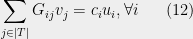
 :
:
![\displaystyle \sum_{i\in[|S|]}G_{ij}u_{i} = d_{j}v_{j}, \forall j \ \ \ \ \ (13)](https://s0.wp.com/latex.php?latex=%5Cdisplaystyle++%5Csum_%7Bi%5Cin%5B%7CS%7C%5D%7DG_%7Bij%7Du_%7Bi%7D+%3D+d_%7Bj%7Dv_%7Bj%7D%2C+%5Cforall+j++%5C+%5C+%5C+%5C+%5C+%2813%29&bg=eeeeee&fg=000000&s=0&c=20201002)
Definition 13 (Solution Algebra) A solution algebra
 consists of self-adjoint (Hermitian) operators
  that satisfy the following predicates:

![\displaystyle (\sum_{j\in[|T|]}G_{ij}X_{j})^{2} = (c_{i})^{2}\cdot\mathbb{I}, \forall i \ \ \ \ \ (15)](https://s0.wp.com/latex.php?latex=%5Cdisplaystyle++%28%5Csum_%7Bj%5Cin%5B%7CT%7C%5D%7DG_%7Bij%7DX_%7Bj%7D%29%5E%7B2%7D+%3D+%28c_%7Bi%7D%29%5E%7B2%7D%5Ccdot%5Cmathbb%7BI%7D%2C+%5Cforall+i++%5C+%5C+%5C+%5C+%5C+%2815%29&bg=eeeeee&fg=000000&s=0&c=20201002) XOR game G (with no zero rows or columns) and a solution algebra , a collection of Linear Operators
XOR game G (with no zero rows or columns) and a solution algebra , a collection of Linear Operators  and density matrix
  are the marginal of an optimal strategy iff the map
  induces a density-matrix representation of and commutes with
  .
Put simply, the theorem states that our unknown self-adjoint operators map to an optimal marginal strategy iff the density matrix (traced from the joint Hilbert-Space) commutes with all the mapped operators (). The result we desire on the lower bound for the number of entangled bits, given a mapping from these indeterminate operators to the marginal of an optimal strategy, comes from a corollary to (14).
.
Put simply, the theorem states that our unknown self-adjoint operators map to an optimal marginal strategy iff the density matrix (traced from the joint Hilbert-Space) commutes with all the mapped operators (). The result we desire on the lower bound for the number of entangled bits, given a mapping from these indeterminate operators to the marginal of an optimal strategy, comes from a corollary to (14).
Corollary 15 Given a
XOR game G (with no zero rows or columns) and a solution algebra with minimum dimension  among non-zero representations, the strategy for minimum entanglement uses
  entangled bits.
The proof for this corollary follows from the eigenspace decomposition of the joint Hilbert Space
entangled bits.
The proof for this corollary follows from the eigenspace decomposition of the joint Hilbert Space  in terms of , which is preserved by the action of
  . As a result, each eigenspace decomposes into a finite sum of irreducible representations of
  . The minimum entanglement is realized when there is exactly one invariant subspace (with one irreducible representation). The entanglement used by such a representation is
  .
.
Proof of Theorem 20
The rest of the section is dedicated to sketching a brief (but formal) proof for Theorem (14), and then using a simple fact about the representations of a Clifford Algebra to show how Slofstra’s result subsumes Tsirelson’s bound. For this section, refers to an arbitrary state in
  (the joint Hilbert space). We can write
  over some basis
  , where
  is a linear map. Then, the partial trace of over is given by
  .
Let
.
Let  denote the algebra generated by
  and
and  . Here, the generating elements are the observables of an optimal quantum strategy.
To arrive at a proof for the theorem, we will rely on 2 additional lemmas which we will not prove but state.
. Here, the generating elements are the observables of an optimal quantum strategy.
To arrive at a proof for the theorem, we will rely on 2 additional lemmas which we will not prove but state.
Lemma 16 Given Hermitian operators
,  ,
,


 with all
  , and we use the second lemma to show that the closure of is
  .
We first show the forward direction:
Suppose we are given an optimal quantum strategy (
.
We first show the forward direction:
Suppose we are given an optimal quantum strategy ( ) for a game . Then, we fix our optimal vector strategy as:

 , and apply Lemma (16) to show commutativity and Lemma (17) to show that = cyclic(
 ).
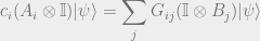
Using (13) with (20) and (21), we have:
).
Using (13) with (20) and (21), we have:
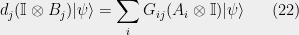 on (22) to see that commutes with every
  .
Additionally, as the terms in (22) constitute linear combinations of
.
Additionally, as the terms in (22) constitute linear combinations of  and , we can compute the closure of their actions on
  and
and  , which will be equivalent. Therefore,
  = , which follows from the special case of (19).
For the dual case, we substitute (20) and (21) into (12):
= , which follows from the special case of (19).
For the dual case, we substitute (20) and (21) into (12):
satisfy predicate (15) making them the representations of  :
:
 This shows that the map from
  computes a density matrix representation of , where commutes with all .
Backward Direction : The proof for the backward direction is much less involved: If we knew that
 constituted the cyclic representation of with commutativity (with ), then we can use Lemma (19) to conclude that the image of on would form a subspace of
  . We define:
 allowing us to recover our original marginal biases
  that satisfy (23) and therefore correspond to the optimal strategy. This shows us that
  , would constitute an optimal quantum strategy.
Lemma 18 For a Clifford Algebra generated by
 , there exist one or two irreducible representations of dimension
  Plugging Lemma 18 into Corollary 15, we simply recover the fact that the number of entangled bits of a solution algebra that is Clifford is . However, note that being Clifford means an extra constraint:
 ,
,  The constraints on the Solution Algebra (14), (15) given by Slofstra do \textit{not} necessarily mean that the solution is Clifford. In fact, when an optimal quantum strategy with minimal entanglement is Clifford, , are constructed from a unique set of
  ,
,  .
To end, we write down a lemma that shows there exist XOR games where the optimal strategy is not unique and for minimal entanglement, a solution generated by a Non-Clifford algebra must be used:
.
To end, we write down a lemma that shows there exist XOR games where the optimal strategy is not unique and for minimal entanglement, a solution generated by a Non-Clifford algebra must be used:
Lemma (Existence of XOR games with Non-Clifford optimal strategies)
There exist a family of XOR games
  that correspond to generalizations of the CHSH games (
 ), such that, the optimal strategy of minimal entanglement is Non-Clifford.
References
[1] David Avis, Sonoko Moriyama, and Masaki Owari. From bell inequalities to tsirelson’s theorem. IEICE Transactions, 92-A(5):1254–1267, 2009.
[2] Lance Fortnow, John Rompel, and Michael Sipser. On the power of multi-prover interactive protocols. Theoretical Computer Science, 134(2):545 – 557, 1994.
[3] T. Ito, H. Kobayashi, and K. Matsumoto. Oracularization and Two-Prover One-Round Interactive Proofs against Nonlocal Strategies. ArXiv e-prints, October 2008.
[4] J. Kempe, H. Kobayashi, K. Matsumoto, B. Toner, and T. Vidick. Entangled games are hard to approximate. ArXiv e-prints, April 2007.
[5] Julia Kempe, Oded Regev, and Ben Toner. Unique games with entangled provers are easy. SIAM Journal on Computing, 39(7):3207– 3229, 2010.
[6] S. Khanna, M. Sudan, L. Trevisan, and D. Williamson. The approximability of constraint satisfaction problems. SIAM Journal on Computing, 30(6):1863–1920, 2001.
[7] Anand Natarajan and Thomas Vidick. Two-player entangled games are NP-hard. arXiv e-prints, page arXiv:1710.03062, October 2017.
[8] Anand Natarajan and Thomas Vidick. Low-degree testing for quantum states, and a quantum entangled games PCP for QMA. arXiv e-prints, page arXiv:1801.03821, January 2018.
[9] William Slofstra. Lower bounds on the entanglement needed to play xor non-local games. CoRR, abs/1007.2248, 2010.
[10] B.S. Tsirelson. Quantum analogues of the bell inequalities. the case of two spatially separated domains. Journal of Soviet Mathematics, 36(4):557–570, 1987.
[11] Thomas Vidick. Three-player entangled XOR games are NP-hard to approximate. arXiv e-prints, page arXiv:1302.1242, February 2013.
[12] Thomas Vidick. Cs286.2 lecture 15: Tsirelson’s characterization of xor games. Online, December 2014. Lecture Notes.
[13] Thomas Vidick. Cs286.2 lecture 17: Np-hardness of computing 
