by Jeremy Dohmann, Vanessa Wong, Venkat Arun
Abstract
We will discuss error-correcting codes: specifically, low-density parity-check (LDPC) codes. We first describe their construction and information-theoretical decoding thresholds, 
Belief propagation (BP) (see Tom’s notes) can be used to decode these. We analyze BP to find the maximum error-rate upto which BP succeeds.
After this point, BP will reach a suboptimal fixed point with high probability. This is lower than the information-theoretic bound, illustrating a gap between algorithmic and information-theoretic thresholds for decoding.
Then we outline a proof of a theorem suggesting that any efficient algorithm, not just BP, will fail after the algorithmic threshold. This is because there is a phase transition at the algorithmic threshold, after which there exist an exponentially large number of suboptimal `metastable’ states near the optimal solution. Local search algorithms will tend to get stuck at these suboptimal points.
Introduction to Error Correcting Codes
Motivation
Alice wants to send a message to Bob, but their channel of communication is such that Bob receives a corrupted version of what Alice sent. Most practical communication devices are imperfect and introduce errors in the messages they are transmitting. For instance, if Alice sends 3V, Bob will really receive three volts plus some noise (we have chosen to ignore some inconvenient practical details here). In many cases, this noise is quite small, e.g. it could be less than 0.5V in 99.99% of cases. So, in principle, Alice could have had very reliable delivery by just choosing to always send 0V for a logical 0 and 5V for logical 1, using checksums to detect the occasional error. But this is wasteful. Alice could have squeezed more levels between 0 and 5V to get a higher bitrate. This causes errors, but Alice can introduce redundancy in the bits she is transmitting which can enable Bob to decode the correct message with high probability. Since it is much easier to control redundancy in encoding than in physical quantities, practical communication devices often choose choose to pack enough bits into their physical signal that errors are relatively quite likely, relying instead on redundancy in their encoding to recover from the errors. Redundancy is also used in storage, where we don’t have the option of detecting an error and retransmitting the message.
Some errors in communication are caused by thermal noise. These are unpredictable and unavoidable, but the errors they cause can be easily modeled; they cause bit-flips in random positions in the message. There are other sources of error. The clocks on the two devices may not be correctly synchronized, causing systematic bit-flips in a somewhat predictable pattern. A sudden surge of current (e.g. because someone turned on the lights, and electricity sparked between the contacts) can corrupt a large contiguous segment of bits. Or the cable could simply be cut in which case no information gets through. These other kinds of errors are often harder to model (and easier to detect/mitigate), so we have to remain content with merely detecting them. Thus for the remainder of this blog post, we shall restrict ourselves to an error model where each bit is corrupted with some fixed (but potentially unknown) probability, independent of the other bits. For simplicity, we shall primarily consider the Binary Erasure Channel (BEC), where a bit either goes through successfully, or the receiver knows that there has been an error (though we will introduce some related channels along the way).
Claude Shannon found that given any channel, there is a bitrate below which it is possible to communicate reliably with vanishing error rate. Reliable communication cannot be achieved above this bitrate. Hence this threshold bitrate is called the channel capacity. He showed that random linear codes are an optimal encoding scheme that achieves channel capacity. We will only briefly discuss random linear codes, but essentially they work by choosing random vectors in the input space and mapping them randomly to vectors in the encoded space. Unfortunately we do not have efficient algorithms for decoding these codes (mostly due to the randomness in their construction), and it is conjectured that one doesn’t exist. Recently Low-Density Parity Check (LDPC) codes have gained in popularity. They are simple to construct, and can be efficiently decoded at error levels quite close to the theoretical limits.
With LDPC codes, there are three limits of interest for any given channel and design bitrate (M/N): 1) the error level upto which an algorithm can efficiently decode them, 


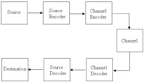
More formally, information theory concerns reliable communication via an unreliable channel. To mitigate the errors in message transmission, error correcting codes introduce some type of systematic redundancy in the transmitted message. Encoding maps are applied to the information sequence to get the encoded message that is transmitted through the channel. The decoding map, on the other hand, is applied to the noisy channel bit (see Figure below). Each message encoded is comprised of 


Claude Shannon’s code ensembles proved that it is easier to construct stochastic (characterized by good properties and high probability) models vs. deterministic code designs. Stochastic models were able to achieve optimal error correcting code performance in comparison to a more rigidly constructed model, proving that it was possible to communicate with a vanishing error probability as long as the rate of transmission 
Thus, in order to construct an optimal error correcting code, one must first define the subset of the space of encoding maps, endow the set with probability distributions, and subsequently define the associated decoding map for each of the encoding maps in the codes. We have included a section in the A that gives a thorough discussion of random code ensembles which are known to achieve optimal decoding, whether via scoring decoding success by bit error rate or decoded word error rate. We will also show a perspective which uses principles from statistical physics to unify the two (often called finite-temperature decoding). From hereon out we will discuss LDPC and explore how the values of
Low-density Parity Check Code
LDPC codes are linear and theoretically excellent error correcting codes that communicate at a rate close to the Shannon capacity. The LDPC codebook is a linear subspace of 


where all the multiplications and sums involved in 
Matrix 


Every coding scheme has three essential properties that determine its utility: the geometry of its codebook and the way it sparsely distributes proper codewords within the encoding space 
A coding scheme over a given channel (whether it be BSC, BEC, AWGN, etc.) also has three parameters of interest, 

LDPC codebook geometry and
On the subject of codebook geometry, it is well known that LDPC ensembles, in expectation, produce sparsely distributed codewords. This means that valid codewords (i.e. those that pass all parity checks) are far apart from one another in Hamming space and thus require a relatively large number of bits to be lost in order for one codeword to degenerate into another one. There is an important property called the distance enumerator which determines the expected number of codewords in a tight neighborhood of any given codeword. If for a given distance the expected number is exponentially small, then the coding scheme is robust up to error rates causing that degree of distortion. We discuss a proof of LDPC distance properties in Appendix B and simply state here that LDPCs are good at sparsely distributing valid codewords within the encoding space. The property
The information theoretic threshold,
Every LDPC ensemble has some different
We will not derive the
Ease of construction
On the subject of ease of construction and ease of decoding, there is a much simpler graphical representation of LDPC codes which can be used to demonstrate LDPC tractability.
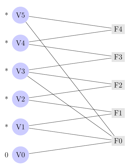
LDPCs can be thought of as bipartite regular graphs, where there are N variable nodes which are connected to M parity check nodes according to randomly chosen edges based on the degree distribution of the LDPC. Though the appendix discusses general degree distributions we will discuss here only (d,k) regular bipartite graphs, in which all variables have d edges and all parity check nodes have k edges, and how to generate them under the configuration model.
The configuration model can be used to generate a bipartite graph with (d,k) degree distribution by initially assigning all variable nodes d half-edges, all parity check nodes k half-edges, and then randomly linking up half-edges between the two sets, deleting all nodes which end up being paired an even number of times, and collapsing all odd numbered multi-edges into a single edge. This system doesn’t work perfectly but for large N, the configuration model will generate a graph for which most nodes have the proper degree. Thus it is relatively easy to generate random graphs which represent LDPC codes of any desired uniform degree distribution. An example of this graphical representation is in figure 2

How the graphical model relates to fast decoding
The graphical model of LDPCs is useful because it is both easy to construct and presents a natural way to perform fast decoding. In fact, the fast graph-based decoding algorithm, Belief Propagation, we use has a
We have seen recently that bipartite graphical models
which represent a factorized probability distribution can be used to calculate marginal probabilities of individual variable nodes (what a mouthful!).
Basically, if the structure of the graph reflects some underlying probability distribution (e.g. the probability that noisy bit 


This is important because when we perform decoding, we would like to estimate the marginal probability of each individual variable node (bit in our received vector), and simply set the variable to be the most likely value (this is known as bit-MAP decoding, discussed earlier). As mentioned above, under certain conditions the Belief Propagation algorithm correctly calculates those marginal probabilities for noise rates up to an algorithmic threshold
The Belief Propagation algorithm is an iterative message passing algorithm in which messages are passed between variable nodes and parity check/factor nodes such that, if the messages converge to a fixed point, the messages encode the marginal probabilities of each variable node. Thus BP, if it succeeds can perform bit-MAP decoding and thus successfully decode.
We will show in the next section how the configuration model graphs map to a factorized probability distribution and mention the
Decoding Errors via Belief Propagation
As mentioned above (again, please see Tom’s excellent blog post for details), the belief propagation algorithm is a useful inference algorithm for stochastic models and sparse graphs derived from computational problems exhibiting thresholding behavior. As discussed, symbol/bit MAP decoding of error correcting codes can be regarded as a statistical inference problem. In this section, we will explore BP decoding to determine the threshold for reliable communication and according optimization for LDPC code ensembles in communication over a binary input output symmetric memoryless channel (BSC or BMS).
Algorithm Overview
Recall that the conditional distribution of the channel input 


Where 


Furthermore

is an indicator variable which takes value 
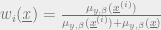
We would like to design a message passing scheme such that the incoming messages for a given variable node encode their marginal probabilities 
Note, first and foremost that this probability can be factorized a la BP factor graphs such that there is a factor node for each parity check node 
and a factor node for each channel probability term
The message passing scheme ends up taking the form


Where 

Messages are passed along the edges as distributions over binary valued variables described by the log-likelihoods


We also introduce the a priori log likelihood for bit

Once we parametrize the messages as log-likelihoods, it turns out we can rewrite our update rules in terms of the parametrized values h and u, making updates much simpler:
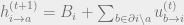

Given a set of messages, we would perform decoding via the overall log likelihood 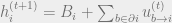


Typically BP is run until it converges to a set of messages that decode to a word in the codebook, or until a max number of iterations have occurred. Other stopping criteria exist such as the messages between time step t and t+1 being all within some small 
It is important to note some properties of BP:
- BP always terminates in
steps if the factor graph is a tree of depth
- It is not known under what circumstances so called “loopy” BP will converge for non-tree graphs
Because factor graphs of LDPC codes are relatively sparse, they appear “locally tree-like”, a property which is believed to play a crucial role in BP convergence over the factorized probability distribution used in LDPC MAP decoding (eqn 1). As mentioned above BP manages to converge on many sorts of non tree-like graphs given that they have “nice” probability distributions. For example the SK model is known to converge even though the underlying factor graph is a complete graph!
It turns out that BP converges under some noise levels for LDPC decoding, and that the threshold at which it fails to converge,
In appendix C we will show some important properties of BP. The following tables summarize important results for several ensembles and channels. Note how close the information theoretic threshold for LDPCs is to the actual shannon limit
Table 1: Thresholds for BSC
Various thresholds for BP over LDPC codes in a Binary Symmetric Channel
| d | k | | | Shannon limit |
| 3 | 4 | .1669 | .2101 | .2145 |
| 3 | 5 | .1138 | .1384 | .1461 |
| 3 | 6 | .084 | .101 | .11 |
| 4 | 6 | .1169 | .1726 | .174 |
See Mezard and Montanari, 2009 Chapt 15. for this table
Table 2: Thresholds for BEC
Various thresholds for BP over LDPC codes in a Binary Erasure Channel
| d | k |  |  | Shannon limit |
| 3 | 4 | .65 | .746 | .75 |
| 3 | 5 | .52 | .59 | .6 |
| 3 | 6 | .429 | .4882 | .5 |
| 4 | 6 | .506 | .66566 | .6667 |
See Mezard and Montanari, 2009 Chapt 15. for this table
We will now show exact behavior of the (3,6) LDPC ensemble over the binary erasure channel.
Algorithmic Thresholds for Belief Propagation (BP)
Definitions and notation
Definition 1. In a Binary Erasure Channel (BEC), when the transmitter sends a bit 


For BECs, the Shannon capacity—the maximum number of data bits that can be transmitted per encoded bit—is given by
Definition 2. An 


For ease of discourse, we have refrained from defining ECC in full generality.
Definition 3. An 


In an LDPC code, 


BP/Peeling algorithm
In general, decoding can be computationally hard. But there exists an error rate 


Belief propagation (BP) for decoding LDPC-codes is equivalent to a simple peeling algorithm. Let us first describe the factor-graph representation for decoding. This is denoted in figure 3. Variables on the left are the received symbol 
BP/the peeling algorithm works as follows. For simplicity of exposition, consider that the all zeros code-word has been transmitted. Since this is a linear code, there is no loss of generality. At first, only the
BP isn’t perfect
This algorithm is not perfect. Figure 3 is an example of a received codeword which can be unambiguously decoded — only the all zeros codeword satisfies all the constraints— but the BP algorithm fails, because at any point, all factor nodes have more than one unknown variable. It seems that the only way to solve problems like that is to exhaustively understand the implications of the parity-check equations. If this examples seems contrived, that is because it is. Decoding becomes harder as the degree and number of constraints increases; we had to add a lot of constraints to make this example work. Fortunately, if the graph is sparse, BP succeeds. We prove this in the following theorem:
Phase transitions for BP
Theorem 1. A 
![\epsilon_d = \mathrm{inf}_{z \in (0, 1)}\left[\frac{z}{\lambda(1 - \rho(1 - z))}\right]](https://s0.wp.com/latex.php?latex=%5Cepsilon_d+%3D+%5Cmathrm%7Binf%7D_%7Bz+%5Cin+%280%2C+1%29%7D%5Cleft%5B%5Cfrac%7Bz%7D%7B%5Clambda%281+-+%5Crho%281+-+z%29%29%7D%5Cright%5D&bg=eeeeee&fg=666666&s=0&c=20201002)
Proof. To prove this, let us analyze the density evolution. For BECs, this is particularly simple as we only need to keep track of the fraction of undetermined variables and factor nodes at timestep 


The first holds because a variable node is undetermined at timestep 


A similar reasoning holds for the second relation. 


Composing the two relations in equation 8, we get the recursion:

An example of 


The condition for BP to converge is 
For (3, 6) regular graphs, 
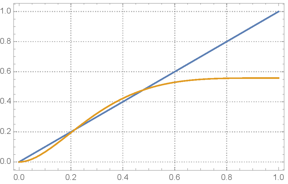
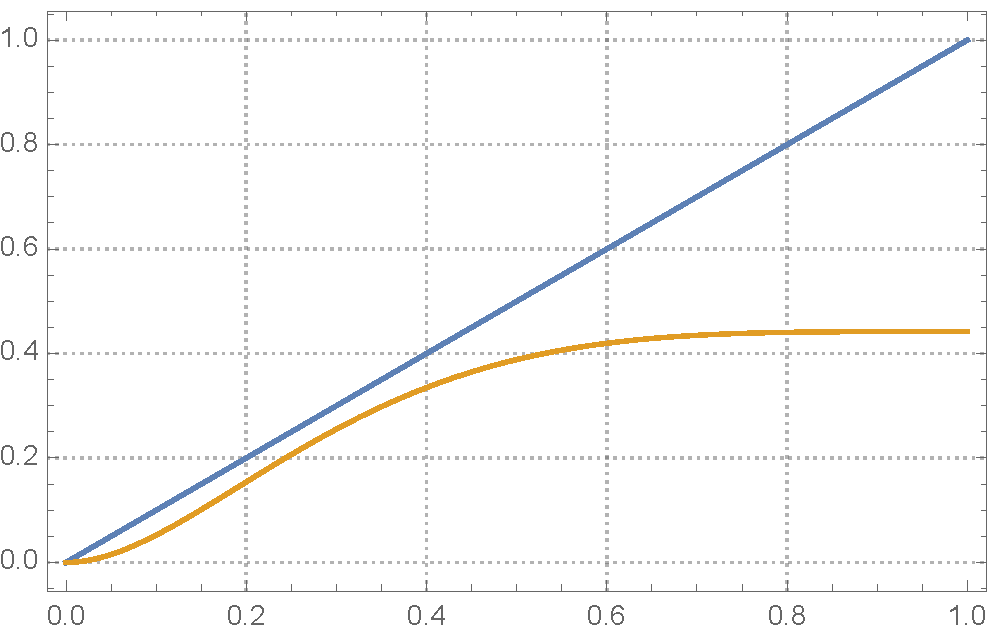
Fig 4 The recursion relation for a (3,6) regular graph, where
 is plotted against . The identity function is also shown (in blue). Here
  . The graph above and below show the case the error rate is below and above respectively.
Another interesting phase transition can be observed. As 
To see the gap between 


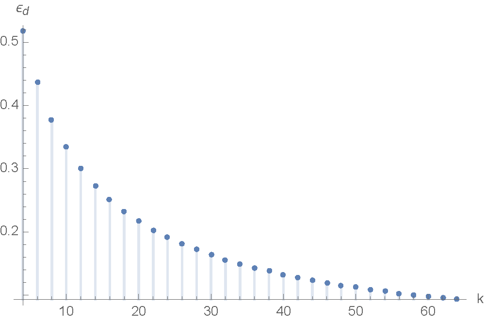 decreases as
  increases, while the rate
  is fixed. In fact
  .
.Finally we would like to mention that it is possible to choose a sequence of polynomials
The solution space in 
The energy landscape of LDPC decoding
We have already shown the exact location of the 
It should not be surprising to us that any given algorithm we attempt to throw at the problem fails at a certain point below
What is of interest to us here, is that
In this section we will rephrase decoding as an energy minimization problem and use three techniques to explore the existence of metastable states and their effect on local search algorithms.
In particular we will first use a generic local search algorithm that attempts to approximately solve energy minimization expression of decoding.
We will next use a more sophisticated Markov chain Monte Carlo method called simulated annealing. Simulated annealing is useful because it offers a perspective that more closely models real physical processes and that has the property that its convergence behavior closely mimics the structure of the metastable configurations.
Energy minimization problem
To begin, we will reframe our problem in terms of constraint satisfaction.
The codewords of an LDPC code are solutions of a CSP. The variables are the bits of the word and the constraints are the parity check equations. Though this means our constraints are a system of linear equations, our problem here is made more complicated by the fact that we are searching for not just ANY solution to the system but for a particular solution, namely the transmitted codeword.
The received message 
Assume we are using the binary-input, memoryless, output-symmetric channel with transition probability 
The probability that 
Where

We can associate an optimization problem with this code. In particular, define 
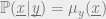
We have already discussed how symbol MAP computes the marginals of the distribution 
We shall here discuss two related problems
- optimizing the energy function within a subset of the configuration space defined by the received word
- sampling from a ’tilted’ Boltzmann distribution associated with the energy
Define the log-likelihood of x being the input given the received y to be

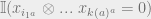
If we assume WLOG that the all zero codeword was transmitted, by the law of large numbers, for large N the log-likelihood 


This suggests that we should look for the transmitted codeword amongst those 
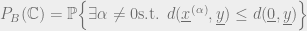
The constraint version of our decoding strategy – known as typical-pairs decoding – is thus, find 
Since codewords are global energy minima (
Minimize
This decoding succeeds iff the minimum is non-degenerate. This happens with high probability for 

Similar to what we have seen elsewhere in the course, there exists a generically intermediate regime
What is so special about BP is that the threshold at which these exponentially many metastable states proliferate is exactly the algorithmic threshold

 (the transmitted codeword) and no local minima. Center: many deep local minima appear, although the global minimum is non degenerate. Right: more than one codeword is compatible with the likelihood constraint, the global minimum is degenerate adapted from Mezard and Montanari, 2009 Chapt 21
While finding solutions
We will show that if one resorts to local-search-based algorithms, the metastable states above
Below is the simplest of local search algorithms, 

Delta search typefies local search algorithms. It walks semi-randomly through the landscape searching for low energy configurations. Its parameter is defined such that, when stuck in a metastable state it can climb out of it in polynomial time if the steepness of its energy barrier is 

MCMC and the relaxation time of a random walk
We can understand the geometry of the metastable states in greater detail by reframing our MAP problem as follows:

This form is referred to as the `tilted’ Boltzmann because it is a Boltzmann distribution biased by the likelihood function.
In the low temperature limit this reduces to eqn 10 because it finds support only over words in the codebook.
This distribution more closely mimics physical systems. For nonzero temperature it allows support over vectors which are not actually in our codebook but still have low distance to our received message and have low energy – this allows us to probe the metastable states which trap our local algorithms. This is referred to as a code with `soft’ parity check constraints as our distribution permits decodings which fail some checks.
We will use the following algorithm excerpted from Mezard and Montanari Chapt 21:
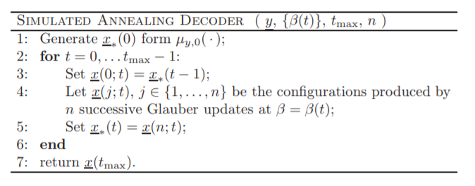
Where a Glauber update consists of scanning through the bits of the current proposed configuration and flipping the value of bit
Where 
This method is a spin-off of traditional Markov chain Monte-Carlo algorithms with the variation that we lower the temperature according to an annealing schedule that initially assigns probability to all states proportional to the likelihood component of equation 12, allowing the chain to randomly sample the configuration space in the neighborhood of the received noisy word, until in the low temperature limit it becomes concentrated near to configurations which are proper codewords.
This method is useful to us because MCMCs are good models of how randomized methods of local searching for optimal configurations occurs in physical systems. Furthermore, the convergence of MCMCs and the time it takes them to converge tells us both the properties of the energy wells they terminate in and the barriers between minima in the energy landscape.
Let’s now show a property relating convergence times of MCMCs and energy barriers known as the Arrhenius law.
If we take the example of using a simple MCMC random walk with the update rule below over the following landscape
![w(x\rightarrow x') = min \{e^{-\beta [E(x')-E(x)]},~1\}](https://s0.wp.com/latex.php?latex=w%28x%5Crightarrow+x%27%29+%3D+min+%5C%7Be%5E%7B-%5Cbeta+%5BE%28x%27%29-E%28x%29%5D%7D%2C%7E1%5C%7D&bg=eeeeee&fg=666666&s=0&c=20201002)

 . Excerpted from Mezard and Montanari, 2009 Chapt 13
We find that the expected number of time steps to cross from one well to another is governed by the Arrhenius law 
In general, if there exists a largest energy barrier between any two components of the configuration space (also known as the bottleneck) the time it takes to sample both components, also known as the relaxation time of the MCMC is
With this in mind, we can apply our simulated annealing MCMC to LDPC decoding and examine the properties of the bottlenecks, or metastable states, in our configuration landscape.
Exact values of the metastable energy states for the BEC
It is a well-known consequence of the 1RSB cavity method that the number of metastable states of energy 


Neglecting the actual form of the calculations I will show the following approximate results for the BEC.

 and
and  . Left: the complexity function as a function of energy density above . Right: the maximum and minimum energy densities of metastable states as a function of the erasure probability. Note that at
  latex the curve is positive only for non zero metastable energy densities. This indicates exponentially many metastable states. At erasure rates above there are exponentially many degenerate ground states. Excerpted from Mezard and Montanari, 2009 Chapt 21
In the regime 
As the error rate of the channel increases above 


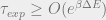
 , and the annealing schedule consists of
  equidistant temperatures in
 ![T = 1 / \beta \in [0,1]](https://s0.wp.com/latex.php?latex=T+%3D+1+%2F+%5Cbeta+%5Cin+%5B0%2C1%5D&bg=eeeeee&fg=666666&s=0&c=20201002) . Left: indicates convergence to the correct ground state at
. Left: indicates convergence to the correct ground state at  . Right: indicates convergence to approximately the energy density of the highest metastable states
  (as calculated by the complexity function via 1RSB) for
  . Excerpted from Mezard and Montanari, 2009 Chapt 21
Here you can see a rough sketch of convergence of the simulated annealing algorithm. As the temperature decreases in the 


Thus we see our local search algorithms end up being attracted to the highest energy of the metastable state.
Excerpted from Mezard and Montanari, 2009 Chapt 21
Though there is not necessarily an exact correspondence between the residual energy at T=0 for simulated annealing and the highest metastable state 
This discussion shows that the algorithmic threshold of BP, 
Appendix A: Random Code Ensembles
In an RCE, encoding maps applied to the information sequence are chosen with uniform probability over a solution space. Two decoding schemes are often used and applied to the noise – word MAP and symbol MAP decoding. MAP, otherwise known as “maximum a priori probability” works by maximizing the probability distribution to output the most probable transmission. Word MAP decoding schemes output the codeword with the highest probability by minimizing the block error probability, which is otherwise known as the probability with respect to the channel distribution that the decoded word is different than the true transmitted word. Symbol MAP decoding, on the other hand, minimizes the fraction of incorrect bits averaged over the transmitted code word (bit error rate).
RCE code is defined by the codebook in Hamming space, or the set of all binary strings of length 
We look at the performance of RCE code in communication over the Binary Symmetric Channel (BSC), where it is assumed that there is a probability p that transmitted bits will be “flipped” (i.e. with probability p, 1 becomes 0 and 0 becomes 1). With BSCs, channel input and output are the same length N sequences of bits. At larger noise levels, there are an exponential number of codewords closer to
Finite temperature decoding has also been looked at as an interpolation between the two MAP decoding schemes. At low noise, a completely ordered phase can be observed as compared to a glassy phase at higher noise channels. Similar to the a statistical physics model, we can also note an entropy dominated paramagnetic phase at higher temperatures.
Each decoding scheme can be analogized to “sphere packing”, where each probability in the Hamming space distribution represents a sphere of radius r. Decoding schemes have partitions in the Hamming space, so these spheres must be disjoint. If not, intersecting spheres must be eliminated. The lower bound of the remaining spheres is then given by Gilbert-Varshamov bound, whereas the upper bound is dictated by the Hamming distance.
Another random code beside the RCE is the RLC, or random linear code. Encoding in an RLC forms a scheme similar to a linear map, of which all points are equiprobable. The code is specified by an 
There are several sources of randomness in codes. Codes are chosen randomly from an ensemble and the codeword to be transmitted is chosen with uniform probability from the code, according to the theorem of source-channel separation. The channel output is then distributed according to a probabilistic process accounting for channel noise and decoding is done by constructing another probability distribution over possible channel inputs and by estimating its signal bit marginal. The decision on the i-th bit is dependent on the distribution. Thus, complications may arise in distinguishing between the two levels of randomness: code, channel input, and noise (“quenched” disorder) versus Boltzmann probability distributions.
Appendix B: Weight enumerators and code performance
The geometric properties of the LDPC codebooks is given by studying the distance enumerator 


denoting an ‘annealed average’, or a disordered system that could be dominated by rare instances in the ensemble. This gives an upper bound on the number of ‘colored factor graphs’ that have an even number of weighted incident edges divided by the total number of factor graphs in the ensemble.
On the other hand, for graphs of fixed degrees with N variable nodes of degree l and M function nodes of degree k, the total number of edges F is given by 


If we aim to join variable and check nodes so that colorings are matched, knowing that there are 

At low noise limits, code performance depends on the existence of codewords at distances close to the transmitted codeword. Starting with degree 1 and knowing that the parametric representation for weights is given by
derive that

when 


or that the number of codewords around a particular codeword is 


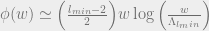
suggesting that LDPC codes with this property have good short distance behavior. Thus, any error that changes a fraction of the bits smaller than 

Let us now focus on the capacity of LDPC codes to correct typical errors in a probabilistic channel. For binary symmetric channels that flip each transmitted bit independently with probability 


This derivation proves that the block error probability depends on the weight enumerator and the 


Appendix C: BP performance
See figure 2 for an illustration of a factor graph illustrating this relationship. Again, recall that for LDPC code ensembles in large block-length limits, the degree distributions of variable nodes and check nodes are given by 


Symmetry
Symmetry of channel log-likelihood and the variables appearing in density evolution are attributes of a desired BMS channel, suggesting that symmetry is preserved by BP operations in evolution. If we assume that the factor graph associated with an LDPC code is “tree-like”, we can apply BP decoding with a symmetric random initial condition and note that the messages 


Physical degradation
Let’s first define physical degradation with BMS channels. If we take two channels BMS(1) and BMS(2) denoted by transition matrices


This is analogous to a Markov chain 
Thresholds
We then fix a particular LDPC code and look at BP messages as random variables due to randomness in the vector
Proposition: If 


Density evolution in this manner is a useful estimate of the number of distributions of density evolution variables 


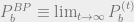
![p_{d} \equiv \sup \Big\{ p \in [0,1/2] : P_b^{BP}(p)=0 \Big\}](https://s0.wp.com/latex.php?latex=p_%7Bd%7D+%5Cequiv+%5Csup+%5CBig%5C%7B+p+%5Cin+%5B0%2C1%2F2%5D+%3A+P_b%5E%7BBP%7D%28p%29%3D0+%5CBig%5C%7D&bg=eeeeee&fg=666666&s=0&c=20201002)
For 


References
[1] Marc Mezard and Andrea Montanari.
Information, Physics, and Computation.
Oxford Graduate Texts, 2009.
