Belief Propagation and the Stochastic Block Model

[Guest post by Thomas Orton who presented a lecture on this in our physics and computation seminar –Boaz]

Introduction

This blog post is a continuation of the CS229R lecture series. Last week, we saw how certain computational problems like 3SAT exhibit a thresholding behavior, similar to a phase transition in a physical system. In this post, we’ll continue to look at this phenomenon by exploring a heuristic method, belief propagation (and the cavity method), which has been used to make hardness conjectures, and also has thresholding properties. In particular, we’ll start by looking at belief propagation for approximate inference on sparse graphs as a purely computational problem. After doing this, we’ll switch perspectives and see belief propagation motivated in terms of Gibbs free energy minimization for physical systems. With these two perspectives in mind, we’ll then try to use belief propagation to do inference on the the stochastic block model. We’ll see some heuristic techniques for determining when BP succeeds and fails in inference, as well as some numerical simulation results of belief propagation for this problem. Lastly, we’ll talk about where this all fits into what is currently known about efficient algorithms and information theoretic barriers for the stochastic block model.

(1) Graphical Models and Belief Propagation

(1.0) Motivation

Suppose someone gives you a probabilistic model on $\vec{x}=(x_1,...,x_n) \in \chi^{N}$ (think of $\chi$ as a discrete set) which can be decomposed in a special way, say

$P(\vec{x})\propto \prod_{a \in F} f_{a}(\vec{x})$

where each $f_{a}$ only depends on the variables $V_{a}$ . Recall from last week that we can express constraint satisfaction problems in these kinds of models, where each $f_{a}$ is associated with a particular constraint. For example, given a 3SAT formula $\phi=\land_{a} c_{a}$ , we can let $f_{a}(\vec{x})=1$ if $c_{a}(\vec{x})$ is satisfied, and 0 otherwise. Then each $f_{a}$ only depends on 3 variables, and $P(\vec{x})$ only has support on satisfying assignments of $\phi$ .

A central problem in computer science is trying to find satisfying assignments to constraint satisfaction problems, i.e. finding values $\vec{x}$ in the support of $P(\vec{x})$ . Suppose that we knew that the value of $P(x_1=1)$ were $>0$ . Then we would know that there exists some satisfying assignment where $x_1=1$ . Using this knowledge, we could recursively try to find $\vec{x}$ ‘s in the support of $P(1,x_2,...,x_n)$ , and iteratively come up with a satisfying assignment to our constraint satisfaction problem. In fact, we could even sample uniformally from the distribution as follows: randomly assign $x_1$ to $1$ with probability $P(x_1=1)$ , and assign it to $0$ otherwise. Now iteratively sample from $P(x_2|x_1)$ for the model where $x_1$ is fixed to the value we assigned to it, and repeat until we’ve assigned values to all of the $\{x_i\}_{i}$ . A natural question is therefore the following: When can we try to efficiently compute the marginals

$P(x_i):=\sum_{\vec{x}-x_i} P(\vec{x})$

for each $i$ ?

A well known efficient algorithm for this problem exists when the corresponding graphical model of $P(\vec{x})$ (more in this in the next section) is a tree. Even though belief propagation is only guaranteed to work exactly for trees, we might hope that if our factor graph is “tree like”, then BP will still give a useful answer. We might even go further than this, and try to analyze exactly when BP fails for a random constraint satisfaction problem. For example, you can do this for k-SAT when $k$ is large, and then learn something about the solution threshold for k-SAT. It therefore might be natural to try and study when BP succeeds and fails for different kinds of problems.

(1.1) Deriving BP

We will start by making two simplifying assumptions on our model $P(\vec{x})$ .

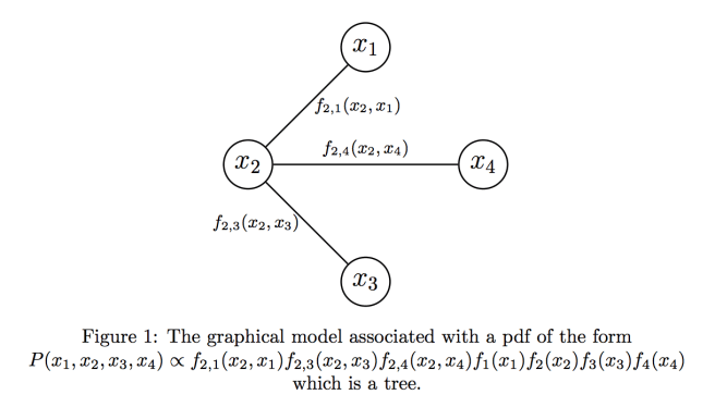
First, we will assume that $P(\vec{x})$ can be written in the form $P(\vec{x})\propto \prod_{(i,j) \in E} f_{i,j}(x_i,x_j) \prod_{i \in [n]} f_i(x_i)$ for some functions $\{f_{i,j}\}_{i,j}, \{f_i(x_i)\}_{i}$ and some “edge set” $E$ (where the edges are undirected). In other words, we will only consider pairwise constraints. We will see later that this naturally corresponds to a physical interpretation, where each of the “particles” $x_i$ interact with each other via pairwise forces. Belief propagation actually still works without this assumption (which is why we can use it to analyze $k$ -SAT for $k>2$ ), but the pairwise case is all we need for the stochastic block model.

For the second assumption, notice that there is a natural correspondence between $P(\vec{x})$ and the graphical model $T$ on $n$ vertices, where $(i,j)$ forms an edge in $T$ iff $(i,j) \in E$ . In order words, edges $(i,j)$ in $T$ correspond to factors of the form $f_{i,j}$ in $P(\vec{x})$ , and vertices in $T$ correspond to variables in $\vec{x}$ . Our second assumption is that the graphical model $T$ is a tree.

graphical_model_fig_1

Now, suppose we’re given such a tree $T$ which represents our probabilistic model. How to we compute the marginals? Generally speaking, when computer scientists see trees, they begin to get very excited [reference]. “I know! Let’s use recursion!” shouts the student in CS124, their heart rate noticeably rising. Imagine that we arbitrarily rooted our tree at vertex $x_i$ . Perhaps, if we could somehow compute the marginals of the children of $x_i$ , we could somehow stitch them together to compute the marginal $x_i$ . In order words, we should think about computing the marginals of roots of subtrees in our graphical model. A quick check shows that the base case is easy: suppose we’re given a graphical model which is a tree consisting of a single node $x_i$ . This corresponds to some PDF $P(\vec{x})=P(x_i) \propto f_{i}(x_i)$ . So to compute $P(x_i)$ , all we have to do is compute the marginalizing constant $Z=\sum_{x_i \in \chi} f_{i}(x_i)$ , and then we have $P(x_i)=\frac{1}{Z}f(x_i)$ . With the base case out of the way, let’s try to solve the induction step: given a graphical model which is a tree rooted at $x_i$ , and where we’re given the marginals of the subtrees rooted at the children of $x_i$ , how do we compute the marginal of the tree rooted at $x_i$ ? Take a look at figure 2 to see what this looks like graphically. To formalize the induction step, we’ll define some notation that will also be useful to us later on. The main pieces of notation are $T^{i \rightarrow j}$ , which is the subtree rooted at $x_i$ with parent $x_j$ , and the “messages” $\psi^{k \rightarrow i}_{x_i}$ , which can be thought of as information which is passed from the child subtrees of $x_i$ to the vertex $x_i$ in order to compute the marginals correctly.

We let $\partial i$ denote the neighbours of vertex $i$ in $T$ . In general, I’ll interchangeably switch between vertex $i$ and the variable $x_i$ represented by vertex $i$ .
We define $T^{i \rightarrow j}$ to be the subtree of $T$ rooted at $i$ , where $i$ ‘s parent is $j$ . We need to specify $i$ ‘s parent in order to give an orientation to our tree (so that we know in which direction we need to do recursion down the tree). Likewise, we let $V_{i \rightarrow j}$ be the set of vertices/variables which occur in subtree $T^{i \rightarrow j}$ .
We define the function $T^{i \rightarrow j}(V_{i \rightarrow j})$ , which is a function of the variables in $V_{i \rightarrow j}$ , to be equal to the product of $T^{i \rightarrow j}$ ‘s edges and vertices. Specifically, $T^{i \rightarrow j}(V_{i \rightarrow j})=\prod_{(a,b) \in E'} f_{a,b}(x_a,x_b) \prod_{a \in V_{i \rightarrow j}} f_{a}(x_a)$ , where $E'$ is the set of edges which occur in subtree $T^{i \rightarrow j}$ . We can think of $T^{i \rightarrow j}(V_{i \rightarrow j})$ as being the pdf (up to normalizing constant) of the “model” of the subtree $T^{i \rightarrow j}$ .
Lastly, we define $\psi^{i \rightarrow j}_{x_i}:=\frac{1}{Z^{i \rightarrow j}} \sum_{V_{i \rightarrow j}-x_i} T(V_{i \rightarrow j})$ , where $Z^{i \rightarrow j}$ is a normalizing constant chosen such that $\sum_{x_i \in \chi} \psi^{i \rightarrow j}_{x_i}=1$ . In particular, $\psi^{i \rightarrow j}_{x_i}: \chi \rightarrow \mathbb{R}$ is a function defined for each possible value of $x_i \in \chi$ . We can interpret $\psi^{i \rightarrow j}_{x_i}$ in two ways: firstly, it is the marginal of the root of the subtree $T^{i \rightarrow j}$ . Secondly, we can think of it as a “message” from vertex $i$ to vertex $j$ . We’ll see why this is a valid interpretation shortly.

graphical_model_recursion

Phew! That was a lot of notation. Now that we have that out of the way, let’s see how we can express the marginal of the root of a tree as a function of the marginals of its subtrees. Suppose we’re considering the subtree $T^{i \rightarrow j}$ , so that vertex $i$ has children $(\partial i)-j$ . Then we can compute the marginal $\psi^{i \rightarrow j}_{r}$ directly:

eqs_1

The non-obvious step in the above is that we’re able to switch around summations and products: we’re able to do this because each of the trees are functions on disjoint sets of variables. So we’re able to express $\psi^{i \rightarrow j}_{x_i}$ as a function of the children values $\{\psi^{k \rightarrow i}_{x_k}\}_{k \in \partial i-j}$ . Looking at the update formula we have derived, we can now see why the $\{\psi^{k \rightarrow i}_{x_k}\}_{k \in \partial i-j}$ are called “messages” to vertex $i$ : they send information about the child subtrees to their parent $i$ .

The above discussion is a purely algebraic way of deriving belief propagation. A more intuitive way to get this result is as follows: imagine fixing the value of $x_i=a$ in the the subtree $T^{i \rightarrow j}$ , and then drawing from each of the marginals of the children of $x_i$ conditioned on the value $x_i=a$ . We can consider the marginals of each of the children independently, because the children are independent of each other when conditioned on the value of $x_i$ . Converting words to equations, this means that if $x_i$ has children $x_{k_{1}},...,x_{k_{d}}$ , then the marginal probability of $(x_i,x_{k_{1}},...,x_{k_{d}})$ in the subtree $T^{i \rightarrow j}$ is proportional to 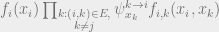$f_{i}(x_i) \prod_{\substack{k:(i,k) \in E, \\ k \not = j}} \psi^{k \rightarrow i}_{x_k} f_{i,k}(x_i,x_k)$ . We can then write

$\psi_{x_i}^{i \rightarrow j} \propto \sum_{(\partial i)-j} f_{i}(x_i) \prod_{\substack{k:(i,k) \in E, \\ k \not = j}} \psi^{k \rightarrow i}_{x_k} f_{i,k}(x_i,x_k)$

$= f_{i}(x_i)\prod_{\substack{k:(i,k) \in E, \\ k \not = j}} \sum_{x_k \in \chi} \psi^{k \rightarrow i}_{x_k} f_{i,k}(x_i,x_k)$

And we get back what we had before. We’ll call this last equation our “update” or “message passing” equation. The key assumption we used was that if we condition on $x_i$ , then the children of $x_i$ are independent. It’s useful to keep this assumption in mind when thinking about how BP behaves on more general graphs.

A similar calculation yields that we can calculate the marginal of our original probability distribution $\psi_{x_i}^{i}:=P(x_i)$ as the marginal of the subtree with no parent, i.e.

$\psi_{x_i}^{i} \propto f_{i}(x_i)\prod_{k:(i,k) \in E} \sum_{x_k \in \chi} \psi^{k \rightarrow i}_{x_k} f_{i,k}(x_i,x_k)$

Great! So now we have an algorithm for computing marginals: recursively compute $\psi^{i \rightarrow j}_{x_i}$ for each $(i,j) \in E$ in a dynamic programming fashion with the “message passing” equations we have just derived. Then, compute $\psi_{x_i}^{i}$ for each $i \in [n]$ . If the diameter of our tree $T$ is $d$ , then the recursion depth of our algorithm is at most $d$ .

However, instead of computing every $\psi^{i \rightarrow j}_{x_i}$ neatly with recursion, we might try something else: let’s instead randomly initialize each $\psi^{i \rightarrow j}_{x_i}$ $(x_i \in \chi)$ with anything we want. Then, let’s update each $\psi^{i \rightarrow j}_{x_i}$ in parallel with our update equations. We will keep doing this in successive steps until each $\psi^{i \rightarrow j}_{x_i}$ has converged to a fixed value. By looking at belief propagation as a recursive algorithm, it’s easy to see that all of the $\psi^{i \rightarrow j}_{x_i}$ ‘s will have their correct values after at most $d$ steps. This is because (after arbitrarily rooting our tree at any vertex) the leaves of our recursion will initialize to the correct value after 1 step. After two steps, the parents of the leaves will be updated correctly as functions of the leaves, and so they will have the correct values as well. Specifically:
Proposition: Suppose we initialize messages $\psi_{x_i}^{i \rightarrow j}$ arbitrarily, and update them in parallel according to our update equations. If $T$ has diameter $d$ , then after $d$ steps each $\psi_{r}^{i \rightarrow j}$ converges, and we recover the correct marginals.

Why would anyone want to do things in this way? In particular, by computing everything in parallel in steps instead of recursively, we’re computing a lot of “garbage” updates which we never use. However, the advantage of doing things in this way is that this procedure is now well defined for general graphs. In particular, suppose $P(\vec{x})$ violated assumption (2), so that the corresponding graph were not a tree. Then we could still try to compute the messages $\psi_{x_i}^{i \rightarrow j}$ with parallel updates. We are also able to do this in a local “message passing” kind of way, which some people may find physically intuitive. Maybe if we’re lucky, the messages will converge after a reasonable amount of iterations. Maybe if we’re even luckier, they will converge to something which gives us information about the marginals $\{P(x_i)\}_{i}$ . In fact, we’ll see that just such a thing happens in the stochastic block model. More on that later. For now, let’s shift gears and look at belief propagation from a physics perspective.

(2) Free Energy Minimization

(2.0) Potts model (Refresh of last week)

We’ve just seen a statistical/algorithmic view of how to compute marginals in a graphical model. It turns out that there’s also a physical way to think about this, which leads to a qualitatively similar algorithm. Recall from last week that another interpretation of a pairwise factor-able PDF is that of particles interacting with each other via pairwise forces. In particular, we can imagine each particle $x_i$ interacting with $x_j$ via a force of strength

$J_{(i,j)}(x_i,x_j)$

and in addition, interacting with an external field

$h_{i}(x_i)$

We imagine that each of our particles take values from a discrete set $\chi$ . When $\chi=\{0,1\}$ , we recover the Ising model, and in general we have a Potts model. The energy function of this system is then

$E[\vec{x}]=-\sum_{(i,j)}J_{(i,j)}(x_i,x_j)-\sum_{i}h_{i}(x)$

with probability distribution given by

$P(\vec{x})=\frac{1}{Z} e^{-E[\vec{x}]/T}$

Now, for $\chi=\{0,1\}$ , computing the marginals $P(x_i)$ corresponds to the equivalent physical problem of computing the “magnetizations” $P(x_i=1)-P(x_i=0)$ .

How does this setup relate to the previous section, where we thought about constraint satisfaction problems and probability distributions? If we could set $e^{-J_{(i,j)}(x_i,x_j)/T}=f_{i,j}(x_i,x_j)$ and $e^{-h_{i}(x_i)/T}=f_{i}(x_i)$ , we would recover exactly the probability distribution 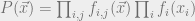$P(\vec{x})=\prod_{i,j} f_{i,j}(\vec{x}) \prod_{i} f_{i}(x_i)$ from the previous section. From a constraint satisfaction perspective, if we set $J_{(i,j)}(x_i,x_j)=1$ if constraint $(i,j)$ is satisfied and $0$ otherwise, then as $T \rightarrow 0$ (our system becomes colder), $P(\vec{x})$ ‘s probability mass becomes concentrated only on the satisfying assignments of the constraint satisfaction problem.

(2.1) Free energy minimization

We’re now going to try a different approach to computing the marginals: let’s define a distribution $b(\vec{x})$ , which we will hope to be a good approximation to $P(\vec{x})$ . If you like, you can think about the marginal $b(x_i)$ as being the “belief” about the state of variable $x_i$ . We can measure the “distance” between $P$ and $b$ by the KL divergence

$KL(b(\vec{x})||p(\vec{x})) =\sum_{\vec{x}}b(\vec{x})\ln\frac{b(\vec{x})}{P(\vec{x})}$

$=\sum_{\vec{x}}b(\vec{x})E(\vec{x})+\sum_{\vec{x}}b(\vec{x})\ln b(\vec{x})+\ln Z$

which equals 0 iff the two distributions are equal. Let’s define the Gibbs free energy as
$G(b(\vec{x}))=\sum_{\vec{x}}b(\vec{x})E(\vec{x})+\sum_{\vec{x}}b(\vec{x})\ln b(\vec{x})=:U(b(\vec{x}))-S(b(\vec{x}))$

So the minimum value of $G$ is $F=-\ln Z$ which is called the Helmholz free energy, $U$ is the “average energy” and $S$ is the “entropy”.

Now for the “free energy minimization part”. We want to choose $b$ to minimize $G$ , so that we can have that $b$ is a good approximation of $P$ . If this happens, then maybe we can hope to “read out” the marginals of $b$ directly. How do we do this in a way which makes it easy to “read out” the marginals? Here’s one idea: let’s try to write $G$ as a function of only the marginals $b(x_i,x_j)$ and $b(x_i)$ of $b$ . If we could do this, then maybe we could try to minimize $G$ by only optimizing over values for “variables” $\{b(x_i,x_j)\}_{i,j}$ and $\{b(x_i)\}_{i}$ . However, we need to remember that $\{b(x_i,x_j)\}_{i,j}$ and $\{b(x_i)\}_{i}$ are actually meant to represent marginals for some real probability distribution $b$ . So at the very least, we should add the consistency constraints $b(x_i)=\sum_{x_j \in \chi} b(x_i,x_j)$ and $\sum_{x_i \in \chi} b(x_i)=1$ to our optimization problem. We can then think of $b(x_i,x_j)$ and $b(x_i)$ as “pseudo-marginals” which obey degree-2 Sherali-Adams constraints.

Recall that we’ve written $G$ as a sum of both the average energy $U$ and the entropy $S$ . It turns out that we can actually write $U$ as only a function of the pariwise marginals of $b$ :

$U(b(\vec{x})) =-\sum_{i,j}\sum_{x_i,x_j} b(x_i,x_j)J_{i,j}(x_i,x_j)-\sum_{i}\sum_{x_i}b(x_i) h_{i}(x_i)$

which follows just because the sums marginalize out the variables which don’t form part of the pairwise interactions:
$\sum_{\vec{x}}b(\vec{x})\left(-\sum_{i,j}J_{i,j}(x_i,x_j)-\sum_{i} h_{i}(x_i)\right)$

$=-\sum_{i,j}\sum_{x_i,x_j} b(x_i,x_j)J_{i,j}(x_i,x_j)-\sum_{i}\sum_{x_i}b(x_i) h_{i}(x_i)$

This is good news: since $P$ only depends on pairwise interactions, the average energy component of $G$ only depends on $b(x_i,x_j)$ and $b(x_i)$ . However, it is not so clear how to express the entropy as a function of one node and two node beliefs. However, maybe we can try to pretend that our model is really a “tree”. In this case, the following is true:

Claim: If our model is a tree, and $\{b(x_i,x_j)\}_{i,j}$ and $\{b(x_i)\}_{i}$ are the associated marginals of our probabilistic model $b(\vec{x})$ , then we have
$b(\vec{x})=\frac{\prod_{(i,j) \in E}b(x_i,x_j)}{\prod_{i \in [n]} b(x_i)^{q_i-1}}$

where $q_i$ is the degree of vertex $x_i$ in the tree.

It’s not too difficult to see why this is the case: imagine a tree rooted at $x_i$ , with children $\partial i$ . We can think of sampling from this tree as first sampling from $x_i$ via its marginal $b(x_i)$ , and then by recursively sampling the children conditioned on $x_i$ . Associate with $\{T_k\}_{k \in \partial i}$ the subtrees of the children of $i$ , i.e. $T_j(V_{j})$ is equal to the probability of the occurrence $V_{j}$ on the probabilistic model of the tree rooted at vertex $j$ . Then we have

$b(\vec{x}) =b(x_i) \prod_{k \in \partial i} b(x_k|x_i) \prod_{k \in \partial i} T_k(V_{k}|x_k)$

$=b(x_i)\frac{1}{b(x_i)^{q_i}} \prod_{k \in \partial i} b(x_i,x_k) \prod_{k \in \partial i}\frac{1}{b(x_k)} \prod_{k \in \partial i}T_k(V_{k})$
$=\frac{\prod_{(i,j) \in E}b(x_i,x_j)}{\prod_{i \in [N]}b(x_i)^{q_i-1}}$

where the last line follows inductively, since each $T_k$ only sees $q_{k}-1$ edges of $x_k$ .

If we make the assumption that our model is a tree, then we can write the Bethe approximation entropy as

$S_{Bethe}=-\sum_{i,j}\sum_{x_i,x_j} b(x_i,x_j)\ln(b(x_i,x_j))+\sum_{i}(q_i-1)\sum_{x_i}b(x_i)\ln b(x_i)$

Where the $\{q_i\}_{i}$ ‘s are the degrees of the variables $\{x_i\}_{i}$ in the graphical model defined by $P(\vec{x})$ . We then define the Bethe free energy as $U+S_{Bethe}$ . The Bethe free energy is in general not an upper bound on the true free energy. Note that if we make the assignments $E_{i}(x_i)=h_{i}(x_i)$ , $E_{i,j}(x_i,x_j)=-J_{i,j}(x_i,x_j)-h_{i}(x_i)-h_{j}(x_j)$ , then we can rewrite $U$ as
$U=\sum_{i,j}\sum_{x_i,x_j} b(x_i,x_j)E_{i,j}(x_i,x_j)+\sum_{i}(q_i-1)\sum_{x_i}b(x_i)E_{i}(x_i)$

which is similar in form to the Bethe approximation entropy. In general, we have

$G_{Bethe}(b(x_i),b(x_i,x_j))=$

$\sum_{i,j}\sum_{x_i,x_j} b(x_i,x_j)(E_{i,j}(x_i,x_j)+\ln(b(x_i,x_j)))$

$-\sum_{i}(q_i-1)\sum_{x_i}b(x_i)( E_{i}(x_i)+\ln b(x_i))$

which is exactly the Gibbs free energy for a probabilistic model whose associated graph is a tree. Since BP gives the correct marginals on trees, we can say that the BP beliefs are the global minima of the Bethe free energy. However, the following is also true:

Proposition: A set of beliefs gives a BP fixed point in any graph (not necessarily a tree) iff they correspond to local stationary points of the Bethe free energy.

(For a proof, see e.g. page 20 of [4])

So trying to minimize the Bethe free energy is in some sense the same thing as doing belief propagation. Apparently, one typically finds that when belief propagation fails to converge on a graph, the optimization program which is trying to minimize $G_{Bethe}$ also runs into problems in similar parameter regions, and vice versa.

(3) The Block Model

(3.0) Definitions

Now that we’ve seen Belief Propagation from two different perspectives, let’s try to apply this technique of computing marginals to analyzing the behavior of the stochastic block model. This section will heavily follow the paper [2].

The stochastic block model is designed to capture a variety of interesting problems, depending on its settings of parameters. The question we’ll be looking at is the following: suppose we generate a random graph, where each vertex of the graph comes from one of $q$ groups each with probability $n_{1},...,n_{q}$ . We add an edge between vertices $(i,j)$ in groups $a,b$ resp. with probability $p_{a,b}$ . For sparse graphs, we define $c_{i,j}:=Np_{i,j}$ , where we think of $p_{i,j}$ as $\mathcal{O}(\frac{1}{N})$ . The problem is the following: given such a random graph, can you label the vertices so that, up to permutation, the labels you choose have high correlation to the true hidden labels which were used to generate the graph? Here are some typical settings of parameters which represent different problems:

Community detection, where we have $q$ groups. We set $n_{i}=\frac{1}{q}$ , and $c_{i,j}=c_{in}$ if $i=j$ and $c_{out}$ otherwise, with $c_{in}>c_{out}$ (assortative structure).
Planted graph partitioning, where $p_{i,j}$ may not necessarily be $\mathcal{O}(\frac{1}{N})$ .
Planted graph colouring, where $p_{in}=0$ , $p_{a,b}=p_{out}$ and $n_{a}=\frac{1}{q}$ for all groups. We know how to efficiently find a planted coloring which is strongly correlated with the true coloring when the average degree $c=(q-1)p_{out}N/q$ is greater than $\mathcal{O}(q^2)$ .

We’ll concern ourselves with the case where our graph is sparse, and we need to try and come up with an assignment for the vertices such that we have high correlation with the true labeling of vertices. How might we measure how well we solve this task? Ideally, a labeling which is identical to the true labeling (up to permutation) should get a score of 1. Conversely, a labeling which naively guesses that every vertex comes from the largest group $\arg \max_{i \in [q]} n_{i}$ should get a score of 0. Here’s one metric which satisfies these properties: if we come up with a labeling $\{t_{i}\}$ , and the true labeling is $\{q_i\}$ , then we’ll measure our performance by

$Q(\{t_{i}\},\{q_{i}\}):=\max_{\pi \in S_q} \frac{\frac{1}{N}\sum_{i \in [N]} \delta_{t_i,\pi(q_i)}-max_{a \in [q]} n_a}{1-\max_{a \in [q]} n_a}$

where we maximize over all permutations $\pi$ . When we choose a labeling which (up to permutation) agrees with the true labeling, then the numerator of $Q$ will equal the denominator, and $Q=1$ . Likewise, when we trivially guess that every vertex belongs to the largest group, then the numerator of $Q$ is $0$ and $Q=0$ .

Given $\{c_{a,b}\},\{n_a\}$ and a set of observed edges $E$ , we can write down the probability of a labeling $\{q_i\}$ as
$P(\{q_i\}_{i})=\prod_{\substack{(i,j) \not \in E \\ i \not = j}}(1-p_{q_{i},q_{j}})\prod_{\substack{(i,j) \in E }}p_{q_{i},q_{j}} \prod_{i \in [q]}n_{q_i}$

How might we try to infer $\{q_i\}$ such that we have maximum correlation (up to permutation) with the true labeling? It turns out that the answer is to use the maximum likelihood estimator of the marginal distribution of each $q_i$ , up to a caveat. In particular, we should label $q_i$ with the $r \in [q]$ such that $P(q_i=r)$ is maximized. The caveat comes in when $P(\{q_i\}_{i})$ is invariant under permutations of the labelings $\{q_i\}_{i}$ , so that each marginal $P(q_i)$ is actually the uniform distribution. For example, this happens in community detection, when all the group sizes $n_{1},...,n_{q}$ are equal. In this case, the correct thing to do is to still use the marginals, but only after we have “broken the symmetry” of the problem by randomly fixing certain values of the vertices to have particular labels. There’s actually a way belief propagation does this implicitly: recall that we start belief propagation by randomly initializing the messages. This random initialization can be interpreted as “symmetry breaking” of the problem, in a way that we’ll see shortly.

(3.1) Belief Propagation

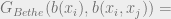
We’ve just seen from the previous section that in order to maximize the correlation of the labeling we come up with, we should pick the labelings which maximize the marginals of $P$ . So we have some marginals that we want to compute. Let’s proceed by applying BP to this problem in the “sparse” regime where $c_{a,b}=Np_{a,b}=\mathcal{O}(1)$ (other algorithms, like approximate message passing, can be used for “dense” graph problems). Suppose we’re given a random graph with edge list $E$ . What does does graph associated with our probabilistic model look like? Well, in this case, every variable is actually connected to every other variable because $P(\{q_i\}_{i})$ includes a factor $f_{i,j}(x_i,x_j)$ for every $(i,j) \in [n] \times [n]$ , so we actually have a complete graph. However, some of the connections between variables are much weaker than others. In full, our BP update equations are

eqs_2

Likewise
$\psi^{i}_{t_{i}}=\frac{1}{Z^{i}} n_{t_{i}} \prod_{\substack{(i,k) \not \in E}}\left[ 1-\frac{1}{N}\sum_{t_k \in [q]}c_{t_1,t_k}\psi^{k \rightarrow i}_{t_k} \right]\prod_{\substack{(i,k) \in E}}\left[\sum_{t_k \in [q]}c_{t_i,t_k} \psi^{k \rightarrow i}_{t_k} \right]$

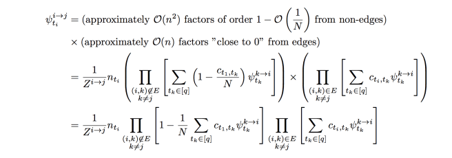
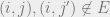what we want to do is approximate these equations so that we only have to pass messages along the edges $E$ , instead of the complete graph. This will make our analysis simpler, and also allow the belief propagation algorithm to run more efficiently. The first observation is the following: Suppose we have two nodes $j,j' \in [N]$ such that $(i,j),(i,j') \not \in E$ . Then we see that $\psi^{i \rightarrow j}_{t_{i}}=\psi^{i \rightarrow j'}_{t_{i}}+\mathcal{O}\left(\frac{1}{N}\right)$ , since the only difference between these two variables are two factors of order $(1-\mathcal{O}\left(\frac{1}{N}\right))$ which appear in the first product of the BP equations. Thus, we send essentially the same messages to non-neighbours $j$ of $i$ in our random graph. In general though, we have:

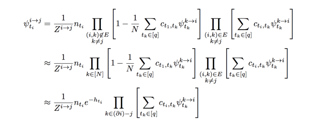
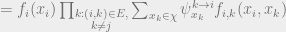
The first approximation comes from dropping non-edge constraints on the first product, and is reasonable because we expect the number of neighbours of $i$ to be constant. We’ve also defined a variable

$h_{t_i}:=\frac{1}{N}\sum_{k \in [N]}\sum_{t_k \in [q]}c_{t_i,t_k} \psi^{k \rightarrow i}_{t_k}$

and we’ve used the approximation $e^{-x} \approx 1-x$ for small $x$ . We think of the term $h_{t_i}$ as defining an “auxiliary external field”. We’ll use this approximate BP equation to find solutions for our problem. This has the advantage that the computation time is $\mathcal{O}(|E|)$ instead of $\mathcal{O}(N^2)$ , so we can deal with large sparse graphs computationally. It also allows us to see how a large dense graphical model with only sparse strong connections still behaves like a sparse tree-like graphical model from the perspective of Belief Propagation. In particular, we might have reason to hope that the BP equations will actually converge and give us good approximations to the marginals.

From now on, we’ll only consider factored block models, which in some sense represent a “hard” setting of parameters. These are models which satisfy the condition that each group has the same average degree $c$ . In particular, we require

$\sum_{d=1}^{q} c_{a,d} n_d = \sum_{d=1}^{q} c_{b,d}n_d =c$

An important observation for this setting of parameters is that

$\psi^{i \rightarrow j}_{t_i}=n_{t_i}$

is always a fixed point of our BP equations, which is known as a factored fixed point (this can be seen by inspection by plugging the fixed point conditions into the belief propagation equations we derived). When BP ever reaches such a fixed point, we get that $Q=0$ and the algorithm fails. However, we might hope that if we randomly initialize $\{\psi^{i \rightarrow j}\}_{(i,j) \in E}$ , then BP might converge to some non-trivial fixed point which gives us some information about the original labeling of the vertices.

(3.2) Numerical Results

Now that we have our BP equations, we can run numerical simulations to try and get a feel of when BP works. Let’s consider the problem of community detection. In particular, we’ll set our parameters with all group sizes $n_{a}$ being equal, and with $c_{a,a}=c_{in}>c_{out}=c_{a,b}$ for $a \not = b$ and vary the ratio $\epsilon:=c_{out}/c_{in}$ , and see when BP finds solutions which are correlated “better than guessing” to the original labeling used to generate the graph. When we do this, we get images which look like this:

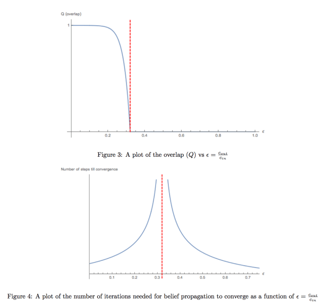
It should be mentioned that the point at which the dashed red line occurs depends on the parameters of the stochastic block model. We get a few interesting observations from numerical experiments:

The point at which BP fails ( $Q=0$ ) happens at a certain value of $\epsilon$ independent of $N$ . In particular, when $\epsilon$ gets too large, BP converges to the trivial factored fixed point. We’ll see in the next section that this is a “stable” fixed point for certain settings of parameters.
Using the approximate BP equations gives the same performance as using the exact BP equations. This numerically justifies the approximations we made.
If we try to estimate the marginals with other tools from our statistical inference toolbox, we find (perhaps surprisingly) that Markov Chain Monte Carlo methods give the same performance as Belief Propagation, even though they take significantly longer to run and have strong asymptotic guarantees on their correctness (if you run MCMC long enough, you will eventually get the correct marginals, but this may take exponential time). This naturally suggests the conjecture that belief propagation is optimal for this task.
As we get closer to the region where BP fails and converges to the trivial fixed point, the number of iterations required for BP to converge increases significantly, and diverges at the critical point $\epsilon_{c}$ where BP fails and converges to the factored fixed point. The same kind of behavior is seen when using Gibbs sampling.

(3.3) Heuristic Stability Calculations

How might we analytically try to determine when BP fails for certain settings of $q$ and $\{c_{a,b}\}$ ? One way we might heuristically try to do this, is to calculate the stability of the factored fixed point. If the fixed point is stable, this suggests that BP will converge to a factored point. If however it is unstable, then we might hope that BP converges to something informative. In particular, suppose we run BP, and we converge to a factored fixed point, so we have that for all our messages $\psi_{t_i}^{i \rightarrow j}=n_{t_i}$ . Suppose we now add a small amount of noise to some of the $\psi_{t_i}^{i \rightarrow j}$ ‘s (maybe think of this as injecting a small amount of additional information about the true marginals). We (heuristically) claim that if we now continue to run more steps of BP, either the messages will converge back to the fixed point $\psi_{t_i}^{i \rightarrow j}=n_{t_i}$ , or they will diverge to something else, and whether or not this happens depends on the eigenvalue of some matrix of partial derivatives.

Following this idea, here’s a heuristic way of calculating the stability of the factored fixed point. Let’s pretend that our BP equations occur on a tree, which is a reasonable approximation in the sparse graph case. Let our tree be rooted at node $k_0$ and have depth $d$ . Let’s try to approximately calculate the influence on $k_0$ of perturbing a leaf $k_d$ from its factored fixed point. In particular, let the path from the leaf to the root be $k_d,...,k_0$ . We’re going to apply a perturbation $\psi^{k_d}_{t} = n_t+\epsilon_{t}^{k}$ for each $t \in [q]$ . In vector notation, this looks like $\psi^{k_d} = \mathbf{1}n_t+\epsilon^{k}$ , where $\psi^{k_d} \in \mathbb{R}^{q \times 1}$ is a column vector. The next thing we’ll do is define the matrix of partial derivatives

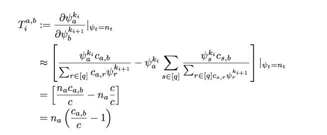
Up to first order (and ignoring normalizing constants), the perturbation effect on $\epsilon^{k_0}$ is then (by chain rule) $\epsilon^{k_0} = \left[\prod_{i=0}^{d-1} T_{i} \right]\epsilon^{k_d}$ . Since $T_{i}$ does not depend on $i$ , we can write this as 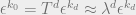$\epsilon^{k_0}=T^{d} \epsilon^{k_d} \approx \lambda^{d} \epsilon^{k_d}$ , where $\lambda$ is the largest eigenvalue of $T$ . Now, on a random tree, we have approximately $c^{d}$ leaves. If we assume that the perturbation effect from each leaf is independent, and that $\epsilon^{k_d}$ has 0 mean, then the net mean perturbation from all the leaves will be 0. The variance will be

if we assume that the cross terms vanish in expectation.

(Aside: You might want to ask: why are we assuming that $\epsilon^{k_{d}}$ has mean zero, and that (say) the noise at each of the leaves are independent, so that the cross terms vanish? If we want to maximize the variance, then maybe choosing the $\epsilon^{k_{d}}$ ‘s to be correlated or have non-zero mean would give us a better bound. The problem is that we’re neglecting the effects of normalizing constants in this analysis: if we perturbed all the $\psi^{k_d}_{t}$ in the same direction (e.g. non-zero mean), our normalization conditions would cancel out our perturbations.)

We Therefore end up with the stability condition $c \lambda^{2} =1$ . When $c \lambda^{2}>1$ , a small perturbation will be magnified as we move up the tree, leading to the messages moving away from the factored fixed point after successive iterations of BP (the fixed point is unstable). If $c \lambda^{2}<1$ , the effect of a small perturbation will vanish as we move up the tree, we expect the factored fixed point to be stable. If we restrict our attention to graphs of the form $c_{a,a}=c_{in}>c_{a,b}=c_{out}$ for $a \not = b$ , and have all our groups with size $n_{a}=\frac{1}{q}$ , then $T$ is known to have eigenvalues $\lambda_{1}=0$ with eigenvector $(1,...,1)$ , and $\lambda_{2}=(c_{in}-c_{out})/qc$ . 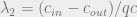The stability threshold then becomes $|c_{in}-c_{out}|=q\sqrt{c}$ . This condition is known as the Almeida-Thouless local stability condition for spin glasses, and the Kesten-Stigum bound on reconstruction on trees. It is also observed empirically that BP and MCMC succeed above this threshold, and converge to factored fixed points below this threshold. The eigenvalues of $T$ are related to the belief propagation equations and the backtracking matrix. For more details, see [3]

(3.4) Information Theoretic Results, and what we know algorithmically

We’ve just seen a threshold for when BP is able to solve the community detection problem. Specifically, when $c<\frac{1}{\lambda^{2}}$ , BP doesn’t do better than chance. It’s natural to ask whether this is because BP is not powerful enough, or whether there really isn’t enough information in the random graph to recover the true labeling. For example, if $c_{out}$ is very close to $c_{in}$ , it might be impossible to distinguish between group boundaries up to random fluctuations in the edges.

It turns out that for $q=2$ , there is not enough information below the threshold $c<\frac{1}{\lambda^{2}}$ to find a labeling which is correlated with the true labeling [3]. However, it can be shown information-theoretically [1] that the threshold at which one can find a correlated labeling is $c_{c} = \Theta \left(\frac{\log(q)}{q \lambda^2} \right)$ . In particular, when $q>11$ , there exists exponential time algorithms which recover a correlated labeling below the Kesten-Stigum threshold. This is interesting, because it suggests an information-computational gap: we observe empirically that heuristic belief propagation seems to perform as well as any other inference algorithm at finding a correlated labeling for the stochastic block model. However, belief propagation fails at a “computational” threshold below the information theoretic threshold for this problem. We’ll talk more about these kinds of information-computation gaps in the coming weeks.

References

[1] Jess Banks, Cristopher Moore, Joe Neeman, Praneeth Netrapalli,
Information-theoretic thresholds for community detection in sparse
networks. AJMLR: Workshop and Conference Proceedings vol 49:1–34, 2016.
Link

[2] Aurelien Decelle, Florent Krzakala, Cristopher Moore, Lenka Zdeborová,
Asymptotic analysis of the stochastic block model for modular networks and its
algorithmic applications. 2013.
Link

[3] Cristopher Moore, The Computer Science and Physics
of Community Detection: Landscapes, Phase Transitions, and Hardness. 2017.
Link

[4] Jonathan Yedidia, William Freeman, Yair Weiss, Understanding Belief Propogation and its Generalizations
Link

[5] Afonso Banderia, Amelia Perry, Alexander Wein, Notes on computational-to-statistical gaps: predictions using statistical physics. 2018.
Link

[6] Stephan Mertens, Marc Mézard, Riccardo Zecchina, Threshold Values of Random K-SAT from the Cavity Method. 2005.
Link

[7] Andrea Montanari, Federico Ricci-Tersenghi, Guilhem Semerjian, Clusters of solutions and replica symmetry breaking in random k-satisfiability. 2008.
Link

A big thanks to Tselil for all the proof reading and recommendations, and to both Boaz and Tselil for their really detailed post-presentation feedback.

2 thoughts on “Belief Propagation and the Stochastic Block Model”

A reader says:

October 21, 2018 at 4:25 pm

Thanks for the very interesting exposition.

Some comments:

1. There’s no link to the previous lecture though you refer to it.

2. The first displayed equation is unclear to me. You say you want to “decompose” the probabilistic model. What does a decomposition mean? I understood that it means that the probability P(x) of getting x, is defined to be as the right hand side of the equation. But then the example seems to say that for every satisfying assignment x, it’s probability is 1. Which doesn’t make sense. Where did I get it wrong?

1. 7omj0 says:
  
  October 22, 2018 at 3:16 pm
  
  Thanks for reading it!
  
  1. You’re right. The previous lecture is Tselil’s blog post; I’ll add a link to it shortly. Thanks for pointing that out.
  
  2. Almost: the probability is defined to be proportional (not equal to) the right hand side. So in the example, the probability distribution is uniform over every satisfying assignment. It’s probably worth mentioning that this scenario is very typical of inference tasks: we can easily write down the pdf of a model, but only up to normalizing constant, and the normalizing constant often gives us useful information about the entire distribution. Moreover, calculating the normalizing constant can be computationally hard (in the example for 3SAT, it would be #P complete), and is often a computational problem of interest in many fields (e.g. sampling methods in statistics, models of physical systems, bayesian inference, and computational problems).

	Mostafa Touny on Avi wins the Turing, TCS for…
	Harvard Professors o… on Open letter to the Harvard…
	Harvard Professors o… on Open letter to the Harvard…
	Harvard, we have a p… on Letter to the Harvard Corporat…
	Eitan bachmat on Letter to the Harvard Corporat…

Belief Propagation and the Stochastic Block Model

Introduction

(1) Graphical Models and Belief Propagation

(1.0) Motivation

(1.1) Deriving BP

(2) Free Energy Minimization

(2.0) Potts model (Refresh of last week)

(2.1) Free energy minimization

(3) The Block Model

(3.0) Definitions

(3.1) Belief Propagation

(3.2) Numerical Results

(3.3) Heuristic Stability Calculations

(3.4) Information Theoretic Results, and what we know algorithmically

References

Published by 7omj0

2 thoughts on “Belief Propagation and the Stochastic Block Model”

Leave a comment Cancel reply

Introduction

(1) Graphical Models and Belief Propagation

(1.0) Motivation

(1.1) Deriving BP

(2) Free Energy Minimization

(2.0) Potts model (Refresh of last week)

(2.1) Free energy minimization

(3) The Block Model

(3.0) Definitions

(3.1) Belief Propagation

(3.2) Numerical Results

(3.3) Heuristic Stability Calculations

(3.4) Information Theoretic Results, and what we know algorithmically

References

Share this:

Related

Published by 7omj0

2 thoughts on “Belief Propagation and the Stochastic Block Model”

Leave a comment Cancel reply