Statistical Physics: an introduction in two parts

Statistical physics has deep connections to many computational problems, including statistical inference, counting and sampling, and optimization. Perhaps especially compelling are the field’s insights and intuitions regarding “average-case complexity” and information-computation gaps. These are topics for which the traditional theoretical CS approaches seem ill-suited, while on the other hand statistical physics has supplied a rich (albeit not always mathematically rigorous) theory.

Statistical physics is the first topic in the seminar course I am co-teaching with Boaz this fall, and one of our primary goals is to explore this theory. This blog post is a re-working of a lecture I gave in class this past Friday. It is meant to serve as an introduction to statistical physics, and is composed of two parts: in the first part, I introduce the basic concepts from statistical physics in a hands-on manner, by demonstrating a phase transition for the Ising model on the complete graph. In the second part, I introduce random k-SAT and the satisfiability conjecture, and give some moment-method based proofs of bounds on the satisfiability threshold.

Update on September 16, 3:48pm: the first version of this post contained an incorrect plot of the energy density of the Ising model on the complete graph, which I have amended below.

I. From particle interactions to macroscopic behaviors

In statistical physics, the goal is to understand how materials behave on a macroscopic scale based on a simple model of particle-particle interactions.

For example, consider a block of iron. In a block of iron, we have many iron particles, and each has a net $\{\pm 1\}$ -polarization or “spin” which is induced by the quantum spins of its unpaired electrons. On the microscopic scale, nearby iron atoms “want” to have the same spin. From what I was able to gather on Wikipedia, this is because the unpaired electrons in the distinct iron atoms repel each other, and if two nearby iron atoms have the same spins, then this allows them to be in a physical configuration where the atoms are further apart in space, which results in a lower energy state (because of the repulsion between electrons).

When most of the particles in a block of iron have correlated spins, then on a macroscopic scale we observe this correlation as the phenomenon of magnetism (or ferromagnetism if we want to be technically correct).

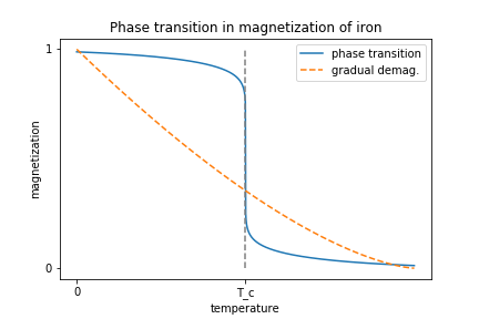
In the 1890’s, Pierre Curie showed that if you heat up a block of iron (introducing energy into the system), it eventually loses its magnetization. In fact, magnetization exhibits a phase transition: there is a critical temperature, $T_c$ , below which a block of iron will act as a magnet, and above which it will suddenly lose its magnetism. This is called the “Curie temperature”. This phase transition is in contrast to the alternative, in which the iron would gradually lose its magnetization as it is heated.

trans

The Ising Model

We’ll now set up a simple model of the microscopic particle-particle interactions, and see how the global phenomenon of the magnetization phase transition emerges. This is called the Ising model, and it is one of the more canonical models in statistical physics.

Suppse that we have $n$ iron atoms, and that their interactions are described by the (for simplicity unweighted) graph $G$ with adjacency matrix $A_G$ . For example, we may think of the atoms as being arranged in a 3D cubic lattice, and then $G$ would be the 3D cubic lattice graph. We give each atom a label in $[n] = \{1,\ldots,n\}$ , and we associate with each atom $i \in [n]$ a spin $x_i \in \{\pm 1\}$ .

For each choice of spins or state $x \in \{\pm 1\}^n$ we associate the total energy

$E(x) = - x^\top A_G x= \sum_{(i,j) \in G} - x_i x_j$ .

If two interacting particles have the same spin, then they are in a “lower energy” configuration, and then they contribute $-1$ to the total energy. If two neighboring particles have opposite spins, then they are in a “higher energy” configuration, and they contribute $+1$ to the total energy.

We also introduce a temperature parameter $T$ . At each $T$ , we want to describe what a “typical” configuration for our block of iron looks like. When $T=0$ , there is no kinetic energy in the system, so we expect the system to be in the lowest-energy state, i.e. all atoms have the same spin. As the temperature increases, the kinetic energy also increases, and we will begin to see more anomalies.

In statistical physics, the “description” takes the form of a probability distribution over states $x$ . To this end we define the Boltzmann distribution, with density function $P_{\beta}(x)$ :

$P_{\beta}(x) \propto \exp(-\beta E(x)), \qquad \text{where } \beta = \frac{1}{T}.$

As $T\to 0$ , $\beta\to\infty$ , $P_{\beta}(x)$ becomes supported entirely on the $x$ that minimize $E(x)$ ; we call these the ground states (for connected $G$ these are exactly $x = \pm \vec{1}$ ). On the other hand as $T \to \infty, \beta \to 0$ , all $x \in \{\pm 1\}^n$ are weighted equally according to $P_{\beta}$ .

Above we have defined the Boltzmann distribution to be proportional to $\exp(-\beta E(x))$ . To spell it out,

$P_{\beta}(x) = \frac{1}{Z(\beta)} \exp(-\beta E(x)), \qquad \text{where } Z(\beta) = \sum_{x \in \{\pm 1\}^n} \exp(-\beta E(x)).$

The normalizing quantity $Z(\beta)$ is referred to as the partition function, and is interesting in its own right. For example, from $Z(\beta)$ we can compute the free energy $F(\beta)$ of the system, as well as the internal energy $U(\beta)$ and the entropy $S(\beta)$ :

$F(\beta) = -\frac{1}{\beta} \ln Z(\beta), \qquad \qquad U(\beta) = \frac{\partial}{\partial \beta} (\beta F(\beta)), \qquad \qquad S(\beta) = \beta^2 \frac{\partial}{\partial \beta} F(\beta).$

Using some straightforward calculus, we can then see that $S(\beta)$ is the Shannon entropy,

$S(\beta) = - \sum_{x} P_{\beta}(x)\ln (P_{\beta}(x)),$

that $U(\beta)$ is the average energy in the system,

$U(\beta) = \sum_{x} P_{\beta}(x) \cdot E(x),$

and that the free energy is the difference of the internal energy and the product of the temperature $T = \frac{1}{\beta}$ and the entropy,

$F(\beta) = U(\beta) - T \cdot S(\beta),$

just like the classical thermodynamic definitons!

Why these functions?

The free energy, internal energy, and entropy encode information about the typical behavior of the system at temperature $\beta$ . We can get some intuition by considering the extremes, $\beta \to \infty$ and $\beta \to 0$ .

In cold systems with $\beta \to \infty$ , if we let $E_0$ be the energy of the ground state, $N_0 = |\{x : E(x) = E_0\}|$ be the number of ground state configurations, and $\Delta_E = \min_{x : E(x) \textgreater E_0} E(x) - E_0$ be the energy gap, then

$Z(\beta) = N_0 \exp(-\beta E_0)\cdot\left(1 + O\left(\exp(-\beta \Delta_E)\right)\right),$

where the $O(\cdot)$ notation hides factors that do not depend on $\beta$ . From this it isn’t hard to work out that

$\begin{aligned} F(\beta) &= E_0 -\frac{1}{\beta} \ln(N_0) + O\left(\exp(-\beta \Delta_E)\right),\\ E(\beta) &= E_0 + O\left(\exp(-\beta \Delta_E)\right)\\ S(\beta) &= \ln N_0 + O\left(\exp(-\beta \Delta_E)\right). \end{aligned}$

We can see that the behavior of the system is dominated by the few ground states. As $\beta \to \infty$ , all of the free energy can be attributed to the internal energy term.

On the other hand, as $\beta \to 0$ ,

$\begin{aligned} F(\beta) &= \mathbb{E}_{x\sim\{\pm 1\}^n} E(x) - \frac{n}{\beta} + O(\beta),\\ U(\beta) &= \mathbb{E}_{x\sim\{\pm 1\}^n} E(x) + O(\beta),\\ S(\beta) &= n + O(\beta), \end{aligned}$

and the behavior of the system is chaotic, with the free energy dominated by the entropy term.

Phase transition at the critical temperature.

We say that the system undergoes a phase transition at $\beta_c$ if the energy density $f(\beta) = \lim_{n\to\infty}\frac{1}{n}F(\beta)$ is not analytic at $\beta = \beta_c$ . Often, this comes from a shift in the relative contributions of the internal energy and entropy terms to $F(\beta)$ . Phase transitions are often associated as well with a qualitative change in system behavior.

For example, we’ll now show that for the Ising model with $G = K_n$ the complete graph with self loops, the system has a phase transition at $\beta_c = \frac{1}{2}$ (the self-loops don’t make much physical sense, but are convenient to work with). Furthermore, we’ll show that this phase transition corresponds to a qualitative change in the system, i.e. the loss of magnetism.

Define the magnetization of the system with spins $x$ to be $m(x) = \frac{1}{n}\sum_i x_i$ . If $\lim_{n \to \infty} m(x) \not\to 0$ , then we say the system is magnetized.

In the complete graph, normalized so that the total interaction of each particle is $1$ , there is a direct relationship between the energy and the magnetization:

$E(x) = \frac{1}{n}\sum_{i, j} - x_i x_j = - n\cdot m(x)^2.$

Computing the energy density.

The magnetization takes values $\frac{k}{n}$ for $k\in\{-n,\ldots, n\}$ . So, letting $N_k$ be the number of states with magnetization $k/n$ , we have that

$Z(\beta) = \sum_{x} \exp(-\beta(- n\cdot m(x)^2)) = \sum_{k = -n}^{n} N_k \cdot \exp\left(\beta n \left(\frac{k}{n}\right)^2\right).$

Now, $N_k$ is just the number of strings with Hamming weight $\frac{1}{2}(n+k)$ , so $N_k = \binom{n}{(n+k)/2}$ . By Stirling’s approximation $N_k \approx \exp(n \cdot H(\frac{1+k/n}{2}))$ , where $H$ is the entropy function, so up to lower-order terms

$Z(\beta) \approx \sum_{\substack{k\in [\pm n]\\ k+n \equiv_2 0}} \exp\left( \beta n \left(\frac{k}{n}\right)^2 + H\left(\frac{1 + \frac{k}{n}}{2}\right) n\right).$

Now we apply the following simplification: for $x \in \mathbb{R}^n$ , $\|x\|_{\infty} \le \|x\|_1 \le n \|x\|_{\infty}$ , and then $\log(\|x\|_1) = \log \|x\|_{\infty} + O(\log n)$ . Treating our summands as the entries of the vector $x$ , from this we have,

$\log(Z(\beta)) = \max_{k \in \{-n,\ldots, n\}} \beta n \left(\frac{k}{n}\right)^2 + H\left(\frac{1}{2}\left(1+\frac{k}{n}\right)\cdot n\right) + O\left(\log n\right).$

By definition of the energy density,

$f(\beta) = \lim_{n \to \infty} \left(- \frac{1}{\beta n} \log Z(\beta)\right) = -\lim_{n\to\infty} \max_{k \in \{-n,\ldots, n\}} \left(\frac{k}{n}\right)^2 + \frac{1}{\beta}H\left(\frac{1}{2}(1+\frac{k}{n})\right),$

and since $n \to \infty$ independently of $\beta$ , we also have

$f(\beta) = -\left(\max_{\delta \in [-1,1]} \delta^2 + \frac{1}{\beta}H\left(\frac{1+\delta}{2}\right)\right),$

because the error from rounding $\delta \in [-1,1]$ to the nearest factor of $2/n$ is $O(1/n)$ .

We can see that the first term in the expression for $f(\beta)$ corresponds to the square of the magnetization (and therefore the energy); the more magnetized the system is, the larger the contribution from the first term. The second term corresponds to the entropy, or the number of configurations in the support; the larger the support, the larger the contribution of the second term. As $T = \frac{1}{\beta}\to \infty$ , the contribution of the entropy term overwhelms the contribution of the energy term; this is consistent with our physical intuition.

A phase transition.

We’ll now demonstrate that there is indeed a phase transition in $\beta$ . To do so, we solve for this maximum. Taking the derivative with respect to $\delta$ , we have that

$\frac{\partial}{\partial \delta} \left( \delta^2 + \frac{1}{\beta}H\left(\frac{1+\delta}{2}\right)\right) = 2\delta + \frac{1}{2\beta} \ln \left(\frac{1-\delta}{1+\delta}\right),$

so the derivative is $0$ whenever $\delta = \frac{1}{4\beta} \ln\left(\frac{1+\delta}{1-\delta}\right)$ . From this, we can check the maxima. When $\beta \textgreater \frac{1}{2}$ , there are two maxima equidistant from the origin, corresponding to negatively or positively-magnetized states. When $\beta \textless \frac{1}{2}$ , the maximizer is $0$ , corresponding to an unmagnetized state.

exponent

Given the maximizers, we now have the energy density. When we plot the energy density, the phase transition at $\beta = \frac{1}{2}$ is subtle (an earlier version of this post contained a mistaken plot):

But when we plot the derivative, we can see that it is not smooth at $\beta = \frac{1}{2}$ :

And with some calculus it is possible to show that the second derivative is indeed not continuous at $\beta = \frac{1}{2}$ .

Qualitatively, it is convincing that this phase transition in the energy density is related to a transition in the magnetization (because the maximizing $\delta$ corresponds to the typical magnetization). One can make this formal by performing a similar calculation to show that the internal energy undergoes a phase transition, which in this case is proportional to the expected squared magnetization, $\mathbb{E}_{P_\beta}[-n \cdot m(x)^2]$ .

Beyond the complete graph

The Ising model on the complete graph $K_n$ (also called the Curie-Weiss model) is perhaps not a very convincing model for a physical block of iron; we expect that locality should govern the strength of the interactions. But because the energy and the magnetization are related so simply, it is easy to solve.

Solutions are also known for the 1D and 2D grids; solving it on higher-dimensional lattices, as well as in many other interesting settings, remains open. Interestingly, the conformal bootstrap method that Boaz mentioned has been used towards solving the Ising model on higher-dimensional grids.

II. Constraint Satisfaction Problems

For those familiar with constraint satisfaction problems (CSPs), it may have already been clear that the Ising model is a CSP. The spins $x \in \{\pm 1\}^n$ are Boolean variables, and the energy function $E(x)$ is an objective function corresponding to the EQUALITY CSP on $G$ (a pretty boring CSP, when taken without negations). The Boltzmann distribution gives a probability distribution over assignments to the variables $x$ , and the temperature $T$ determines the objective value of a typical $x \sim P_{\beta}$ .

We can similarly define the energy, Boltzmann distribution, and free energy/entropy for any CSP (and even to continuous domains such as $x \in \mathbb{R}^n$ ). Especially popular with statistical physicists are:

CSPs (such as the Ising model) over grids and other lattices.
Gaussian spin glasses: CSPs over $x \in \{\pm 1\}^n$ or $x \in \mathbb{R}^n$ where the energy function is proportional to $\langle x^{\otimes k}, J\rangle$ , where $J$ is an order- $k$ symmetric tensor with entries sampled i.i.d. from $\mathcal{N}(0,1)$ . The Ising model on a graph with random Gaussian weights is an example for $k = 2$ .
Random instances of $k$ -SAT: Of the $\binom{n}{k} \cdot 2^k$ possible clauses (with negations) on $n$ variables, $m$ clauses $C_1,\ldots,C_m$ are sampled uniformly at random, and the energy function is the number of satisfied clauses, $E(x) = |\{ i \in [m] : C_i(x) = 1\}|$ .
Random instances of other Boolean and larger-alphabet CSPs.

In some cases, these CSPs are reasonable models for physical systems; in
other cases, they are primarily of theoretical interest.

Algorithmic questions

As theoretical computer scientists, we are used to seeing CSPs in the contex of optimization. In statistical physics, the goal is to understand the qualitative behavior of the system as described by the Boltzmann distribution. They ask algorithmic questions such as:

Can we estimate the free energy $F(\beta)$ ? The partition function $Z(\beta)$ ? And, relatedly,
Can we sample from $P_{\beta}$ ?

But these tasks are not so different from optimization. For example, if our system is an instance of 3SAT, when $T=0$ , the Boltzmann distribution is the uniform distribution over maximally satisfying assignments, and so estimating $Z(\infty)$ is equivalent to deciding the SAT formula, and sampling from $P_{\infty}$ is equivalent to solving the SAT formula. As $T$ increases, sampling from $P_{\beta}$ corresponds to sampling an approximate solution.

Clearly in the worst case, these tasks are NP-Hard (and even #P-hard). But even for random instances these algorithmic questions are interesting.

Phase transitions in satisfiability

In random $k$ -SAT, the system is controlled not only by the temperature $T$ but also by the clause density $\alpha = \frac{m}{n}$ . For the remainder of the post, we will focus on the zero-temperature regime $T = 0$ , and we will see that $k$ -SAT exhibits phase transitions in $\alpha$ as well.

The most natural “physical” trait to track in a $k$ -SAT formula is whether or not it is satisfiable. When $\alpha = 0$ , $k$ -SAT instances are clearly satisfiable, because they have no constraints. Similarly when $\alpha = n^k \cdot 2^k$ , random $k$ -SAT instances cannot be satisfiable, because for any set of $k$ variables they will contain all $2^k$ possible $k$ -SAT constraints (clearly unsatisfiable). It is natural to ask: is there a satisfiability phase transition in $\alpha$ ?

For $k = 2$ , one can show that the answer is yes. For $k \ge 3$ , numerical evidence strongly points to this being the case; further, the following theorem of Friedgut gives a partial answer:

Theorem:
For there exists a function $\alpha_c(n)$ such that for any $\epsilon \textgreater 0$ , if $\phi$ is a random $k$ -SAT formula on $n$ variables with $\alpha n$ clauses, then

$\lim_{n \to \infty} \Pr[\phi \text{ is satisfiable}] = \begin{cases} 1 & \text{ if } \alpha \textless (1-\epsilon) \alpha_c(n)\\ 0 & \text{ if } \alpha \textgreater (1+\epsilon) \alpha_c(n) \end{cases}.$

However, this theorem allows for the possibility that the threshold depends on $n$ . From a statistical physics standpoint, this would be ridiculous, as it suggests that the behavior of the system depends on the number of particles that participate in it. We state the commonly held stronger conjecture:

Conjecture:
for all $k \ge 3$ , there exists a constant $\alpha_c$ depending only on $k$ such that if $\phi$ is a random $k$ -SAT instance in $n$ variables and $\alpha n$ clauses, then

$\lim_{n \to \infty} \Pr[\phi \text{ is satisfiable}] = \begin{cases} 1 & \text{ if } \alpha \textless \alpha_c \\ 1 & \text{ if } \alpha \textgreater \alpha_c \end{cases}$

In 2015, Jian Ding, Allan Sly, and Nike Sun established the $k$ -SAT conjecture all $k$ larger than some fixed constant $k_0$ , and we will be hearing about the proof from Nike later on in the course.

Bounds on $\alpha_c$ via the method of moments

Let us move to a simpler model of random $k$ -SAT formulas, which is a bit easier to work with and is a close approximation to our original model. Instead of sampling $k$ -SAT clauses without replacement, we will sample them with replacement and also allow variables to appear multiple times in the same clause (so each literal is chosen uniformly at random). The independence of the clauses makes computations in this model simpler.

We’ll prove the following bounds. The upper bound is a fairly straightforward computation, and the lower bound is given by an elegant argument due to Achlioptas and Peres.

Theorem:
For every $k \ge 3$ , $2^k \ln 2 - O(k) \le \alpha_c \le 2^k \ln 2 - O(1)$ .

Let $\phi$ be a random $k$ -SAT formula with $m = \alpha n$ clauses, $C_1,\ldots,C_m$ . For an assignment $x \in \{\pm 1\}^n$ , let $\phi(x)$ be the $0/1$ indicator that $x$ satisfies $\phi$ . Finally, let $Z_{\alpha} = \sum_x \phi(x)$ be the number of satisfying assignments of $\phi$ .

Upper bound via the first moment method.

We have by Markov’s inequality that

$\Pr[Z_{\alpha} \ge 1] \le \mathbb{E}[Z_{\alpha}] = \sum_{x} \Pr[\phi(x)].$

Fix an assignment $x$ . Then by the independence of the clauses,

$\Pr[\phi(x)] = \prod_{j \in [m]} \Pr[C_j(x) = 1] = \left(1 - \frac{1}{2^k}\right)^m,$

since each clause has $2^k -1$ satisfying assignments. Summing over all
$x \in \{\pm 1\}^n$ ,

$\mathbb{E}[Z_{\alpha}] = 2^n \left(1 - \frac{1}{2^k}\right)^{\alpha n}.$

We can see that if $\alpha \textgreater 2^k \ln 2$ , this quantity will go to $0$ with $n$ . So we have:

$\alpha_c \le 2^k \ln 2.$

Lower bound via the second moment method.

To lower bound $\alpha_c$ , we can use the second moment method. We’ll
calculate the second moment of $Z_{\alpha}$ . An easy use of Cauchy-Schwarz (for non-negative $X$ , $\mathbb{E}[X] \le \sqrt{\mathbb{E}[X^2]\mathbb{E}[I[X \textgreater 0]]}$ ) implies that if there is a constant $c$ such that

$\lim_{n \to \infty}\frac{\left(\mathbb{E} Z_{\alpha}\right)^2}{\mathbb{E}Z_{\alpha}^2} \ge c$ ,

then with at least constant probability $Z_{\alpha} \ge 1$ , and then Friedgut’s theorem implies that $\alpha \textless \alpha_c$ . From above we have an expression for the numerator, so we now set out to bound the second moment of $Z_{\alpha}$ . We have that

$\mathbb{E} Z_{\alpha}^2 = \mathbb{E}\left[\left(\sum_{x}I[\phi(x)]\right)^2\right] = \sum_{x,y} \Pr\left[\phi(x)\wedge \phi(y)\right],$

and by the independence of the clauses,

$\Pr\left[\phi(x)\wedge \phi(y)\right] = \prod_{j \in [m]} \Pr[C_j(x) = 1 \wedge C_j(y) = 1] = \left(\Pr[C(x) = 1 \wedge C(y) = 1]\right)^m,$

for a single random $k$ -SAT clause $C$ . But, for $x,y \in \{\pm 1\}^n$ , the events $C(x) = 1$ and $C(y)=1$ are not independent. This is easier to see if we apply inclusion-exclusion,

$\Pr[C(x) = 1 \wedge C(y) = 1] = 1 - \Pr[C(x) = 0] - \Pr[C(y) = 0] + \Pr[C(x) = C(y) = 0],$

The event that both $C(x) = C(y) = 0$ when $C$ is a $k$ -SAT clause occurs only when $x$ and $y$ agree exactly on the assignments to the variables of $C$ , since otherwise at least one of $x$ or $y$ must be satisfied (because each literal in $C(x)$ is negated for $C(y)$ ). Thus, this probability depends on the Hamming distance between $x$ and $y$ .

agreement

For $x,y$ with $\frac{1}{2}\|x-y\|_1 = (1-\delta)n$ , the probability that $C$ ‘s variables are all in the subset on which $x,y$ agree is $\delta^k$ (up to lower order terms). So, we have

$\Pr[C(x) = C(y) = 0] = \delta^k \cdot \frac{1}{2^k},$

and then for $x,y$ with $\frac{1}{2}\|x-y\|_1 = n - \ell$ ,

$\Pr[C(x) = 1 \wedge C(y) = 1] = 1 - 2\cdot \frac{1}{2^k} + \left(\frac{\ell}{2n}\right)^k.$

Because there are $2^n \cdot \binom{n}{\ell}$ pairs $x,y$ at distance $\frac{1}{2}\|x-y\|_1 = n - \ell$ ,

$\mathbb{E}\left[Z_{\alpha}^2\right] = \sum_{\ell = 0}^{n} 2^n \cdot \binom{n}{\ell} \cdot \left(1 - \frac{1}{2^{k-1}} + \left(\frac{\ell}{2n}\right)^k\right)^m,$

and using the Stirling bound $\binom{n}{\ell} \le O(\frac{1}{\sqrt{n}})\exp(n \cdot H(\ell/n))$ ,

$= \sum_{\ell = 0}^{n}O(\frac{1}{\sqrt{n}}) \exp\left( \left(H\left(\frac{\ell}{n}\right) + \ln 2\right)\cdot n + \ln\left(1 - \frac{1}{2^{k-1}} + \left(\frac{\ell}{2n}\right)^k\right) \cdot \alpha n\right).$

Using Laplace’s method, we can show that this sum will be dominated by the $O(\sqrt{n})$ terms around the maximizing summand; so defining $\psi(\delta) = H(\delta) + \ln 2 + \alpha\ln (1 - 2^{-k+1} + \delta^k 2^{-k}))$ ,

$\mathbb{E}[Z_{\alpha}^2] = O(1) \cdot \exp( n \cdot \max_{\delta \in [0,1]} \psi(\delta)).$

If we want that $\mathbb{E}[Z^2] \le c \cdot \mathbb{E}[Z]^2$ , then we require that

$\max_{\delta \in [0,1]} \psi(\delta) \le \frac{1}{n}\ln(\mathbb{E}[Z]^2) = 2\ln 2 + 2\alpha \ln (1-2^{-k}).$

However, we can see (using calculus) that this inequality does not hold whenever $\alpha \textgreater 0$ . In the plot below one can also see this, though the values are very close when $\alpha$ is close to $0$ :

So the naive second moment method fails to establish any lower bound on $\alpha_c$ . The problem here is that the second moment is dominated by the large correlations of close strings; whenever $\alpha \textgreater 0$ , the sum is dominated by pairs of strings $x,y$ which are closer than $n/2$ in Hamming distance, which is atypical. For strings at Hamming distance $n/2$ , what is relevant is $\psi(\frac{1}{2})$ , which is always

$\psi(\frac{1}{2}) = H(\frac{1}{2}) + \ln 2 + \alpha \ln \left(1 - \frac{1}{2^{k-1}} + \frac{1}{2^{2k}}\right) = 2\ln 2 + \alpha \ln \left(1 - \frac{1}{2^k}\right)^{2},$

which is equal to $\frac{1}{n}\ln\mathbb{E}[Z_{\alpha}]^2$ . At distance $n/2$ , the value of $\phi$ on pairs $x,y$ is essentially uncorrelated (one can think of drawing a uniformly random $y$ given $x$ ), so such pairs are representative of $\mathbb{E}[Z]^2$ .

A more delicate approach.

To get a good bound, we have to perform a fancier second moment method calculation, due to Achlioptas and Peres. We will re-weight the terms so that more typical pairs, at distance $n/2$ , are dominant. Rather than computing $Z_{\alpha}$ , we compute $X_{\alpha}$ , where

$X_{\alpha} = \sum_{x} \prod_{j \in [m]} w_j(x),$

where $w_j(x) = 0$ if $C_j(x) = 0$ , and $w_j(x) = \eta^t$ if $C_j(x)$ is satisfied by $t$ variables. Since $X_{\alpha} \textgreater 0$ only if $\phi$ has satisfying assignments, the goal is to still bound $\mathbb{E}[X_{\alpha}^2] \le c\cdot \mathbb{E}[X_{\alpha}]^2$ . Again using the independence of the clauses, we have that

$\begin{aligned} \mathbb{E}[X_{\alpha}] = 2^n \cdot \mathbb{E}[w_j(x)]^m = 2^n \left(2^{-k}\sum_{t = 1}^k \binom{k}{t} \eta^t \right)^m = 2^n \left(\left(\frac{1+\eta}{2}\right)^k-2^{-k}\right)^m.\label{eq:expect}\end{aligned}$

And calculating again the second moment,

$\mathbb{E}[X_{\alpha}^2] = \sum_{x,y} \prod_{j \in [m]} \mathbb{E}[w_j(x)\cdot w_j(y)].$

For a fixed clause $j$ , we can partition the variables in its scope into 4 sets, according to whether $x,y$ agree on the variable, and whether the variable does or does not satisfy the literals of the clause. Suppose that $w_j$ has $a$ variables on which $x,y$ agree, and that of these $t$ are satisfying for $w_j$ and $a - t$ are not.

agreement-numbers

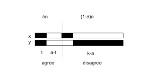
Then, $w_j$ has $k-a$ variables on which $x,y$ disagree, and any variable which does not satisfy $w_j$ for $x$ must satisfy it for $y$ . For a $w_j(x) w_j(y)$ to be nonzero, either there must be at least one literal in the variables on which $x,y$ agree which agrees with $x,y$ , or otherwise there must be at least one literal in the variables on which $x,y$ disagree which agrees with each string. Therefore, if $x,y$ agree on a $\delta$ -fraction of variables,

$\begin{aligned} \mathbb{E}[w_j(x) \cdot w_j(y)] &= \sum_{a = 1}^k \sum_{t=1}^a \eta^{2t + k - a} \cdot \Pr[w_j \text{ has } a \text{ variables in } x \cap y,\ t \in x \cap y \text{ satisfy }w, \ w_j(x),w_j(y) \textgreater 0]\\ &= \left(\sum_{a = 0}^k\sum_{t=0}^a \eta^{k - a + 2t} \cdot \binom{k}{a}\delta^{a}\left(1 - \delta\right)^{k-a} 2^{-a} \binom{a}{t}\right) - \left(\sum_{a=0}^k \eta^{k-a} \binom{k}{a} \delta^a(1-\delta)^{k-a} 2^{-k+1}\right) + \delta^k2^{-k},\end{aligned}$

where the first sum ignores the cases when $w_j(x) = 0$ or $w_j(y) = 0$ , the second sum subtracts for the cases when $t=0$ the contribution of the terms where all the literals agree with either $x$ or $y$ , and the final term accounts for the fact that the term $a = k$ is subtracted
twice. Simplifying,

$\mathbb{E}[w_j(x) \cdot w_j(y)] = \left(\frac{(1+\eta^2)}{2}\delta + \eta(1-\delta)\right)^k - 2^{1-k} \left(\eta(1-\delta) + \delta\right)^k + \left(\frac{\delta}{2}\right)^k.$

Define
$q_{\eta}(\delta) =\left(\frac{(1+\eta^2)}{2}\delta + \eta(1-\delta)\right)^k - 2^{1-k} \left(\eta(1-\delta) + \delta\right)^k + \left(\frac{\delta}{2}\right)^k$ .
So we have (using Laplace’s method again)

$\mathbb{E}[X^2] = 2^n \sum_{\ell = 0}^n \binom{n}{\ell} q_\eta\left(\frac{\ell}{n}\right)^{\alpha n} \approx O(1) \cdot \exp(\max_{\delta \in [0,1]} \psi_\eta (\delta) \cdot n),$

For
$\psi_\eta(\delta) = H(\delta) + \ln 2 + \alpha \ln q_{\eta}(\delta).$

When $\delta = \frac{1}{2}$ ,

$q_{\eta}\left(\frac{1}{2}\right) = \left(\left(\frac{1+\eta}{2}\right)^k - \frac{1}{2^k}\right)^2,$

which is equal to the log of the square of the expectation, so again for the second moment method to succeed, $\delta = \frac{1}{2}$ must be the global maximum.

Guided by this consideration, we can set $\eta$ so that the derivative $q_{\eta}'(\frac{1}{2}) = 0$ , so that $\psi_\eta$ achieves a local maximum at $\delta = \frac{1}{2}$ . The choice for this (after doing some calculus) turns out to be the positive, real solution to the equation 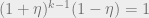$(1+\eta)^{k-1}(1-\eta) = 1$ . With this choice, one can show that the global maximum is indeed achieved at $\delta = \fra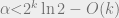c{1}{2}$ as long as $\alpha \textless 2^k \ln 2 - O(k)$ . Below, we plot $\psi_{\eta}$ with this optimal choice of $\eta$ for several values of $\alpha$ at $k = 5$ :

fancy-second-moment

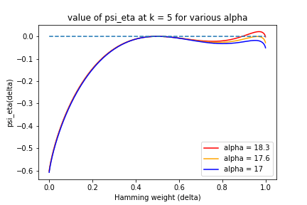
So we have bounded 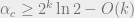$\alpha_c \ge 2^k \ln 2 - O(k)$ .

Another phase transition

What is the correct answer for $\alpha_c$ ? We now have it in a window of size $O(k)$ . Experimental data and heuristic predictions indicate that it is closer to $2^k \ln 2 - O(1)$ (and in fact for large $k$ , Ding, Sly and Sun showed that $\alpha_c$ is a specific constant in the interval $[2^k \ln 2 -2, 2^k \ln 2]$ ). So why can’t we push the second moment method further?

It turns out that there is a good reason for this, having to do with another phase transition. In fact, we know that $k$ -SAT has not only satisfiable and unsatisfiable phases, but also clustering and condensation phases:

ksat-phases

In the clustering phase, there are exponentially many clusters of solutions, each containing exponentially many solutions, and each at hamming distance $\Omega(n)$ from each other. In the condensation phase, there are even fewer clusters, but solutions still exist. We can see evidence of this already in the way that the second moment method failed us. When $\alpha \textgreater 2^k \ln 2 - O(k)$ , we see that the global maximum of the exponent is actually attained close to $\delta = 1$ . This is because solutions with large overlap come to dominate the set of satisfying assignments.

One can also establish the existence of clusters using the method of moments. The trick is to compute the probability that two solutions, $x$ and $y$ with overlap $\delta n$ , are both satisfying for $\phi$ . In fact, we have already done this. From above,

$\Pr\left[\phi(x) \wedge \phi(y) ~\mid~ \frac{1}{2}\|x - y\|_1 = (1-\delta)n\right] = \left(1 - 2\cdot \frac{1}{2^k} + 2^{-k}\delta^k\right)^{\alpha n}.$

Now, by a union bound, an upper bound on the probability that there exists a pair of solutions $x,y$ with overlap $\delta n$ for any $\delta \in [\delta_1,\delta_2]$ is at most

$\Pr[\exists x,y \ s.t. \ \phi(x) \wedge \phi(y), \ \frac{1}{2}\|x-y\|_1 = (1-\delta)n \text{ for } \delta \in [\delta_1,\delta_2]] \le \sum_{\ell = \delta_1 n}^{\delta_2 n} \binom{n}{\ell} \left(1 - 2^{1-k} + \left(\frac{\ell}{2n}\right)^k\right)^{\alpha n}$
$\le \int_{\delta_1}^{\delta_2} \exp\left( \left(H(\delta) + \ln 2 + \alpha \ln \left(1-2^{1-k} + 2^{-k}\delta^k\right)\right)n\right) d\delta,$

and if the function $\beta(\delta) := H(\delta) + \ln 2 + \alpha\ln (1 + 2^{-k}\delta^k - 2^{1-k})$ is such that $\beta(\delta) \textless 0$ for all $\delta \in [\delta_1,\delta_2]$ , then we conclude that the probability that there is a pair of satisfying assignments at distance between $(1-\delta_2)n$ and $(1-\delta_1)n$ is $o(1)$ .

Achlioptas and Ricci-Tersenghi showed that for $k \ge 4$ , $\alpha = (1-\eta)2^k$ , and $\epsilon$ a fixed constant, the above function is less than $0$ . Rather than doing the tedious calculus, we can verify by plotting for $k = 8, \alpha = 169$ (with $169 \textless \alpha_c$ ):

clusters

They also use the second moment method to show the clusters are non-empty, that there are exponentially many of them, each containing exponentially many solutions. This gives a proof of the existence of a clustering regime.

Solution geometry and algorithms

This study of the space of solutions is referred to as solution geometry, and understanding solution geometry turns out to be essential in proving better bounds on the critical density.

Solution geometry is also intimately related to the success of local search algorithms such as belief propagation, and to heuristics for predicting phase transitions such as replica symmetry breaking.

These topics and more to follow, in the coming weeks.

Resources

In preparing this blog post/lecture I leaned heavily on Chapters 2 and 10 of Marc Mézard and Andrea Montanari’s “Information, Physics, and Computation”, on Chapters 12,13,&14 of Cris Moore and Stephan Mertens’ “The nature of Computation,” and on Dimitris Achlioptas and Federico Ricci-Tersenghi’s manuscript “On the Solution-Space Geometry of Random CSPs”. I also consulted Wikipedia for some physics basics.

	Mostafa Touny on Avi wins the Turing, TCS for…
	Harvard Professors o… on Open letter to the Harvard…
	Harvard Professors o… on Open letter to the Harvard…
	Harvard, we have a p… on Letter to the Harvard Corporat…
	Eitan bachmat on Letter to the Harvard Corporat…

Statistical Physics: an introduction in two parts

I. From particle interactions to macroscopic behaviors

The Ising Model

Why these functions?

Phase transition at the critical temperature.

Computing the energy density.

A phase transition.

Beyond the complete graph

II. Constraint Satisfaction Problems

Algorithmic questions

Phase transitions in satisfiability

Bounds on $\alpha_c$ via the method of moments

Upper bound via the first moment method.

Lower bound via the second moment method.

A more delicate approach.

Another phase transition

Solution geometry and algorithms

Resources

Published by tselilschramm

One thought on “Statistical Physics: an introduction in two parts”

Leave a comment Cancel reply

I. From particle interactions to macroscopic behaviors

The Ising Model

Why these functions?

Phase transition at the critical temperature.

Computing the energy density.

A phase transition.

Beyond the complete graph

II. Constraint Satisfaction Problems

Algorithmic questions

Phase transitions in satisfiability

Bounds on via the method of moments

Upper bound via the first moment method.

Lower bound via the second moment method.

A more delicate approach.

Another phase transition

Solution geometry and algorithms

Resources

Share this:

Related

Published by tselilschramm

One thought on “Statistical Physics: an introduction in two parts”

Leave a comment Cancel reply

Bounds on $\alpha_c$ via the method of moments