This is part 4 of a continuing series on clustering, Gaussian mixtures, and Sum of Squares (SoS) proofs. If you have not read them yet, I recommend starting with Part 1, Part 2, and Part 3. Also, if you find errors please mention them in the comments (or otherwise get in touch with me) and I will fix them ASAP.
Last time we finished our SoS identifiability proof for one-dimensional Gaussian mixtures. In this post, we are going to turn it into an algorithm. In Part 3 we proved Lemma 2, which we restate here.
Lemma 2.
Let. Let
be a partition of
into
pieces of size
such that for each
, the collection of numbers
obeys the following moment bound:
where
is the average
and
is a power of
in
. Let
be such that
for every
.
Let
be indeterminates. Let
be the following set of equations and inequalities.
As before
is the polynomial
. Thinking of the variables
as defining a set
via its
indicator, let
be the formal expression
Let
be a degree
pseudoexpectation which satisfies
![w_i^2 = w_i \text{ for } i \in [n]](https://s0.wp.com/latex.php?latex=w_i%5E2+%3D+w_i+%5Ctext%7B+for+%7D+i+%5Cin+%5Bn%5D&bg=eeeeee&fg=666666&s=0&c=20201002)
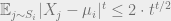
![\sum_{i \in [n]} w_i = N](https://s0.wp.com/latex.php?latex=%5Csum_%7Bi+%5Cin+%5Bn%5D%7D+w_i+%3D+N&bg=eeeeee&fg=666666&s=0&c=20201002)
![\frac 1 N \sum_{i \in [n]} w_i \cdot (X_i - \mu)^t \leq 2 \cdot t^{t/2}.](https://s0.wp.com/latex.php?latex=%5Cfrac+1+N+%5Csum_%7Bi+%5Cin+%5Bn%5D%7D+w_i+%5Ccdot+%28X_i+-+%5Cmu%29%5Et+%5Cleq+2+%5Ccdot+t%5E%7Bt%2F2%7D.&bg=eeeeee&fg=666666&s=0&c=20201002)

![\tilde{\mathbb{E}} \left [ \sum_{i \in [k]} \left ( \frac{|T \cap S_i|}{N} \right ) ^2 \right ] \geq 1 - \frac{2^{O(t)} t^{t/2} k^2}{\Delta^t}.](https://s0.wp.com/latex.php?latex=%5Ctilde%7B%5Cmathbb%7BE%7D%7D+%5Cleft+%5B%C2%A0+%5Csum_%7Bi+%5Cin+%5Bk%5D%7D+%5Cleft+%28+%5Cfrac%7B%7CT+%5Ccap+S_i%7C%7D%7BN%7D+%5Cright+%29+%5E2+%5Cright+%5D+%5Cgeq+1+-+%5Cfrac%7B2%5E%7BO%28t%29%7D+t%5E%7Bt%2F2%7D+k%5E2%7D%7B%5CDelta%5Et%7D.&bg=eeeeee&fg=666666&s=0&c=20201002)
We will we design a convex program to exploit the SoS identifiability proof, and in particular Lemma 2. Then we describe a (very simple) rounding procedure and analyze it, which will complete our description and analysis of the one-dimensional algorithm.
Let’s look at the hypothesis of Lemma 2. It asks for a pseudoexpectation of degree 

It is actually possible to design a rounding algorithm which takes any pseudoexpectation satisfying 
(1) find such a pseudoexpectation
(2) round to find a cluster
(3) remove all the points in 
This is a viable algorithm, but analyzing it is a little painful because misclassifications from early rounds of the rounding algorithm must be taken into account when analyzing later rounds, and in particular a slightly stronger version of Lemma 2 is needed, to allow some error from early misclassifications.
We are going to avoid this pain by imposing some more structure on the pseudoexpectation our algorithm eventually rounds, to enable our rounding scheme to recover all the clusters without re-solving a convex program. This is not possible if one is only promised a pseudoexpectation 


We are going to use a trick reminiscent of entropy maximization to ensure that the pseudoexpectation we eventually round contains information about all the clusters

where 

It may not be so obvious why 


![i \in [k]](https://s0.wp.com/latex.php?latex=i+%5Cin+%5Bk%5D&bg=eeeeee&fg=666666&s=0&c=20201002)

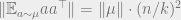
![\|\mathbb{E}_{a \sim \mu} aa^\top \|^2 = \left \langle \sum_{i \in [k]} \mu(a_i) a_i a_i^\top, \sum_{i \in [k]} \mu(a_i) a_i a_i^\top \right \rangle = \sum_{i \in [k]} \mu(a_i)^2 \cdot \|a_i\|^4,](https://s0.wp.com/latex.php?latex=%5C%7C%5Cmathbb%7BE%7D_%7Ba+%5Csim+%5Cmu%7D+aa%5E%5Ctop+%5C%7C%5E2+%3D+%5Cleft+%5Clangle+%5Csum_%7Bi+%5Cin+%5Bk%5D%7D+%5Cmu%28a_i%29+a_i+a_i%5E%5Ctop%2C+%5Csum_%7Bi+%5Cin+%5Bk%5D%7D+%5Cmu%28a_i%29+a_i+a_i%5E%5Ctop+%5Cright+%5Crangle+%3D+%5Csum_%7Bi+%5Cin+%5Bk%5D%7D+%5Cmu%28a_i%29%5E2+%5Ccdot+%5C%7Ca_i%5C%7C%5E4%2C&bg=eeeeee&fg=666666&s=0&c=20201002)
where we have used orthogonality 


We can analyze our convex program via the following corollary of Lemma 2.
Corollary 1.
Let
Let
is the
where
is the Frobenius norm.


Proof of Corollary 1.
The uniform distribution 

We expand the norm:

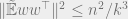
To bound the last term we use Lemma 2. In the notation of that Lemma,
![\langle \tilde{\mathbb{E}} ww^\top, \mathbb{E} aa^\top \rangle = \frac 1k \tilde{\mathbb{E}} \sum_{i \in [k]} |S_i \cap T|^2 \geq \frac 1k \cdot N^2 \cdot \left ( 1 - \frac{2^{O(t)} t^{t/2} k^2}{\Delta^t} \right ).](https://s0.wp.com/latex.php?latex=%5Clangle+%5Ctilde%7B%5Cmathbb%7BE%7D%7D+ww%5E%5Ctop%2C+%5Cmathbb%7BE%7D+aa%5E%5Ctop+%5Crangle+%3D+%5Cfrac+1k+%5Ctilde%7B%5Cmathbb%7BE%7D%7D+%5Csum_%7Bi+%5Cin+%5Bk%5D%7D+%7CS_i+%5Ccap+T%7C%5E2+%5Cgeq+%5Cfrac+1k+%5Ccdot+N%5E2+%5Ccdot+%5Cleft+%28+1+-+%5Cfrac%7B2%5E%7BO%28t%29%7D+t%5E%7Bt%2F2%7D+k%5E2%7D%7B%5CDelta%5Et%7D+%5Cright+%29.&bg=eeeeee&fg=666666&s=0&c=20201002)
Remember that
QED.
We are basically done with the algorithm now. Observe that the matrix 

Once one has in hand a matrix 
We will prove the following fact at the end of this post.
Fact: rounding.
Letbe the
if
and
are in the same cluster
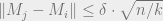
. Suppose $M \in \mathbb{R}^{n \times n}$ satisfies
.
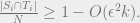
There is a polynomial-time algorithm which takes
and with probability at least
produces a partition
of
such that, up to a permutation of
,
Putting things together for one-dimensional Gaussian mixtures
Now we sketch a proof of Theorem 1 in the case 

then apply the rounding algorithm from the rounding fact to
If the vectors

where

Since a standard Gaussian has 


Rounding algorithm
The last thing to do in this post is prove the rounding algorithm Fact. This has little to do with SoS; the algorithm is elementary and combinatorial. We provide it for completeness.
The setting is: there is a partition 

Let 


The algorithm is:
(1) Let ![\mathcal{I} = [n]](https://s0.wp.com/latex.php?latex=%5Cmathcal%7BI%7D+%3D+%5Bn%5D&bg=eeeeee&fg=666666&s=0&c=20201002)
(2) Pick 
(3) Let 
(4) Add 
(5) If 
(6) (postprocess) Assign remaining indices to clusters arbitrarily, then move indices arbitrarily from larger clusters to smaller ones until all clusters have size
Fact: rounding.
Ifthen with probability at least
.
Proof.
Call an index ![i \in [n]](https://s0.wp.com/latex.php?latex=i+%5Cin+%5Bn%5D&bg=eeeeee&fg=666666&s=0&c=20201002)

![\sum_{i \in [n]} \|M_i - A_i\|^2 = \|M - A\|^2 \leq \epsilon^2 \|A\|^2](https://s0.wp.com/latex.php?latex=%5Csum_%7Bi+%5Cin+%5Bn%5D%7D+%5C%7CM_i+-+A_i%5C%7C%5E2+%3D+%5C%7CM+-+A%5C%7C%5E2+%5Cleq+%5Cepsilon%5E2+%5C%7CA%5C%7C%5E2&bg=eeeeee&fg=666666&s=0&c=20201002)


If 


Consider implementing the algorithm by drawing a list of 


Nice (series of) post(s)!
Two minor details:
* “Frobenious” should read “Frobenius”
* the collision probability is not the $2$-norm of the probability distribution (or rather its pmf), but is the squared $2$-norm