Clustering and Sum of Squares Proofs, Part 1

Update (1/5/18): a pdf containing all six posts in this series is now available on my website.

I am excited to (temporarily) join the Windows on Theory family as a guest blogger!

This is the first post in a series which will appear on Windows on Theory in the coming weeks. The aim is to give a self-contained tutorial on using the Sum of Squares algorithm for unsupervised learning problems, and in particular in Gaussian mixture models. This will take several posts: let’s get started.

In an unsupervised learning problem, the goal is generally to recover some parameters given some data , where is a probability distribution on, say, which is parameterized by . The goal is to estimate by some estimator which (a) does not require too many samples and (b) can be computed from those samples in polynomial time. This basic setup can be instantiated (sometimes with minor adaptations) to capture numerous important problems in statistics and machine learning: a few examples are

•  component analysis and its many variants (PCA, ICA, Sparse PCA, etc.)
• Netflix problem / matrix completion / tensor completion
• dictionary learning / blind source separation
• community detection and recovery / stochastic block models
• many clustering problems

Excellent resources on any of these topics are just a Google search away, and our purpose here is not to survey the vast literature on unsupervised learning, or even on provable “TCS-style” algorithms for these problems. Instead, we will try to give a simple exposition of one technique which has now been applied successfully to many unsupervised learning problems: the Sum of Squares method for turning identifiability proofs into algorithms.

Identifiability is a concept from statistics. If one hopes for an algorithm which recovers parameters , it must at least be true that uniquely (or almost uniquely) determine , with high probability: when this occurs we say is identifiable from the samples .

Classically, identifiability is often proved by analysis of a (typically) inefficient brute-force algorithm. First, one invents some property of . For example, in a maximum-likelihood argument, one shows that for some . Then, often via a concentration-of-measure argument, one shows that no far from satisfies property . In the maximum-likelihood example, this would entail showing that if is far from then .

An identifiability argument like this typically has no implications for computationally-efficient algorithms, since finding which satisfies often appears to require brute-force search. Thus, often when the investigation turns to efficient algorithms, the identifiability argument is abandoned and more explicitly algorithmic techniques are brought to bear: convex relaxations, spectral methods, and even heuristic methods.

The method we present here for designing computationally-efficient algorithms begins with a return to identifiability proofs. The main insight is that if both

• the property and, more importantly,
• the proof that any satisfying must be close to

are sufficiently simple, then identifiability of from does imply the existence of an efficient algorithm to (approximately) recover from !

For us, simple has a formal meaning: the proof should be captured in the low-degree Sum of Squares proof system.

The algorithms which result in the end follow a familiar recipe: solve some convex relaxation whose constraints depend on and round it to obtain . But the design and analysis of this relaxation are heavily informed by the simple identifiability proof described above. In particular, the convex programs which result will not be familiar relaxations of maximum likelihood problems!

In this series of blog posts, we are going to carry out this strategy from start to finish for a classic unsupervised learning problem: clustering mixtures of Gaussians. So that we can get down to business as quickly as possible, we defer a short survey of the literature on this “proofs-to-algorithms” method to a later post.

Mixtures of Gaussians

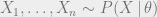
Gaussian mixtures are classic objects in statistics, dating at least to Pearson in 1894. The basic idea is: suppose you have a data set which was generated in a heterogeneous fashion: some points were sampled from probability distribution , some from , and so on up to , but you do not know which points came from which distributions. Under what settings can you cluster the points by which distribution they came from, and perhaps also recover some properties of those distributions, such as their means ?

Pearson, in 1894, was faced with a collection of body measurements of crabs. The distribution of one such attribute in the data — the ratio of forehead length to body width — curiously deviated from a Gaussian distribution. Pearson concluded that in fact two distinct species of crabs were present in his data set, and that the data should therefore be modeled as a mixture of two Gaussians. He invented the method of moments to discover the means of both the Gaussians in question.¹ In the years since, Gaussian mixtures have become a fundamental statistical modeling tool: algorithms to fit Gaussian mixtures to data sets are included in basic machine learning packages like sklearn.

Here is our mixture of Gaussians model, formally.

Mixtures of separated spherical Gaussians:
Let

• .
• be such that for every .
• be -dimensional spherical Gaussians, centered at the means .
• be iid samples, each drawn by selecting uniformly, then drawing .
• be the induced partition of into parts, where if samples was drawn from

The problem is: given , output a partition of into parts, each of size , such that (up to renaming the clusters ),

for each and some small number .

To avoid some minor but notationally annoying matters, we are going to work with a small variant of the model, where we assume that exactly samples came from each Gaussian . We call a mixture like this “equidistributed”.

We will work up to a proof of this theorem, which was proved recently (as of Fall 2017) in 3 independent works.

Main Theorem (Hopkins-Li, Kothari-Steinhardt, Diakonikolas-Kane-Stewart):
For arbitrarily-large there is an algorithm requiring samples from the equidistributed mixtures of Gaussians model and running in time which outputs a partition of into parts of size such that with high probability,

for some universal constant .³

In particular:

• If for some , then by choosing the algorithm recovers the correct clustering up to errors in time with -many samples.
• If for a large-enough universal constant , then choosing gives a quasipolynomial-time algorithm (using quasipolynomially-many samples) to recover clusters up to error.⁴

One (rather weak) consequence of the main theorem is that, for samples, there is enough information in the samples to determine the underlying clustering, up to error . Our strategy to prove the main theorem will start with proving the latter statement independently — as we have discussed, such an argument is often called a proof of identifiability because we say that the clusters are identifiable from the samples (up to errors).

While identifiability itself does not carry immediate algorithmic consequences, our proof of identifiability will be somewhat special: it will be simple in a formal sense, namely, that it will be captured by a formal proof system of restricted power. This simplicity of the proof of identifiability will almost immediately imply the main theorem: the construction of a computationally-efficient algorithm from a simple proof of identifiability is the heart of the proofs-to-algorithms method.

Identifiability proof: 1 dimension

Our eventual goal is to work up to a proof in the low-degree Sum of Squares proof system that clusters are identifiable from samples from a mixture of Gaussians. Since we have not yet defined low-degree Sum of Squares proofs, for now we will focus on constructing an identifiability proof which avoids mathematical facts which we deem “too complicated”. In particular, we will avoid any Chernoff/union bound style arguments.

To get to the heart of the matter it helps to simplify the setting. Our first simplification is to restrict attention to the case, so that distributions are univariate Gaussians with unit variance.

Before stating our first lemma, let’s discuss the key property of a collection of samples from a Gaussian which we will use. Recall that if is a standard Gaussian, then for every ,

If are samples from , then for large enough, the empirical distribution of inherits this property, up to some small fluctuations. Namely, with high probability we would have

(We could have replaced by any small constant greater than .) Here, the notation means that an index is chosen uniformly among .

If for some , then the same discussion applies immediately to and . But even more is true: if is the empirical mean of (that is, ), then with high probability the -th centered empirical moment also inherits the same bound:

In the Gaussian mixture setting, so long as enough samples are drawn from each Gaussian , each cluster will have -th empirical moments satisfying the above bound (with high probability).

In our identifiability proof, we choose to forget that the samples were drawn from Gaussians, and we remember only that they break up into underlying clusters, each of which satisfies that empirical moment bound. We do not even remember the “true” means of each Gaussian; instead we talk only about the empirical means. We will show that no clustering far from that underlying ground-truth clustering results in clusters which satisfy the empirical moment bound.

Lemma 1. Let . Let be a partition of into pieces of size such that for each , the collection of numbers obeys the following moment bound:

where is the average and is some number in . Let be such that for every . Suppose is large enough that .

Let have size and be such that obey the same moment-boundedness property:

for the same , where is the mean . Then there exists an such that

for some universal constant .

How do we interpret Lemma 1 as a statement of cluster identifiability? The lemma implies that the clusters are, up to errors, the only subsets of of size which satisfy the -th moment bound. This is our property , like we discussed earlier in this post. The true clustering satisfies (i.e. if you group by this ground-truth clustering, the resulting clusters will have bounded empirical -th moments), and every clustering which satisfies this bounded -th moment property must be close to the true clustering. Thus, the correct clusters could be identified by searching for subsets of which satisfy the -th moment bound (never mind that such a search would naively require about time).

We said that to use the sum of squares method to turn our identifiability proof into an algorithm, both the property and the proof of identifiability need to be simple.

This -th moment boundedness property will turn out to be simple enough. What about the proof of Lemma 1? By the end of this post we will prove Lemma 1 in a way which uses only Holder’s inequality for the vs norms and the triangle inequality for the -norm. Later, we will show that these inequalities are simple in the correct formal sense: they are captured by a proof system of restricted power.

Our proof of Lemma 1 relies on the following key fact.

Fact 1. Let have . Let denote a uniform sample from and similarly for . Let and . Suppose satisfy the -th moment bound

Then

A slightly more general interpretation of this fact is that a pair of random variables on which have bounded -th moments and whose total variation distance cannot have means which are too far apart: .

Proof of Fact 1.
Let . Observe that there is a coupling of the random variables so that . The coupling chooses with probability to select a uniform sample , then lets . With probability , the random variable is a uniform sample from and similarly for .

Let be a coupled pair of samples. We expand a quantity related to the one we want to bound, and then apply Holder’s inequality with the and norms. (The underlying inner product space assigns functions the inner product .)

Now we can apply the triangle inequality for the -norm to the last term, followed by our -th moment assumptions.

Putting everything together, we get . QED.

Keeping in mind our eventual goal of constructing a low-degree Sum of Squares proof, we record the observation that the only inequalities we required to prove Fact 1 were the vs. Holder’s inequality and the triangle inequality for the -norm.

Armed with Fact 1, we can prove Lemma 1.The main idea in the proof is that if and are the two clusters with greatest intersection with , then can only be close to one of .

Proof of Lemma 1.
Let have size , with mean and -th moment bound . Without loss of generality, order the clusters so that has largest intersection with , then , and so on: that is . If , then , just by counting.

Since , either or . We claim it must be the second. Using Fact 1,

since certainly , and we assumed . We conclude that .

We have obtained and . Putting these together with Fact 1, we find

Rearranging, this reads QED.

Looking ahead

This concludes our one-dimensional identifiability proof, which will form the core of our proof of Theorem 1. In our next post we will lift this proof to a Sum of Squares proof (for which we will need to define Sum of Squares proofs). After that, with a Sum of Squares proof in hand, we will finish designing our mixture of Gaussians algorithm for the one-dimensional case. Then we will show that the same ideas, nearly unchanged, imply that the algorithm works in higher dimensions.

Thanks

Many thanks to Boaz Barak, David Steurer, and especially Daniel Freund for their helpful remarks on early drafts of this post.

Footnotes

1. Moritz Hardt on Gaussian mixtures and Pearson’s approach

2. Image credit: Mathematica Stack Exchange

3. To see how to apply the ideas in this tutorial to a much broader class of clustering problems, see my joint paper with Jerry Li and the recent paper of Pravesh Kothari and Jacob Steinhardt.

4. Before these recent works, the best polynomial-time algorithms for the clustering mixtures of Gaussians could not tolerate any (when a simple greedy algorithm can be shown to solve the clustering problem to high accuracy). On the other hand, known lower bounds show that when , clustering is impossible (even using exponential time) with samples, so one cannot hope to improve the guarantees of this theorem too much further [Regev-Vijayaraghavan]. (That said, reducing the sample complexity and running time to when is a fascinating open problem.)

Variants of this theorem, which may be found in all three of the sources listed, offer algorithms which additionally output estimates of the means , work for many distributions besides Gaussians (without even knowing the underlying distribution!), and tolerate some amount of advesarial corruption among the samples . We note also that the theorems in those works handle the usual mixtures of Gaussians problem, rather than the equidistributed version, and can tolerate non-uniform mixtures; i.e. those where some clusters are much smaller than others.