Clustering and Sum of Squares Proofs, Part 3

This is part 3 of a continuing series on clustering, Gaussian mixtures, and Sum of Squares (SoS) proofs. If you have not read them yet, I recommend starting with Part 1 and Part 2. Also, if you find errors please mention them in the comments (or otherwise get in touch with me) and I will fix them ASAP.

The Story So Far

Let’s have a brief recap. We are designing an algorithm to cluster samples from Gaussian mixture models on $\mathbb{R}^d$ . Our plan is to do this by turning a simple identifiability proof into an algorithm. For us, “simple” means that the proof is captured by the low degree Sum of Squares (SoS) proof system.

We have so far addressed only the case $d = 1$ (which will remain true in this post). In part 1 we designed our identifiability proof, not yet trying to formally capture it in SoS. The proof was simple in the sense that it used only the triangle inequality and Holder’s inequality. In part 2 we defined SoS proofs formally, and stated and proved an SoS version of one of the key facts in the identifiability proof (Fact 2).

In this post we are going to finish up our SoS identifiability proof. In the next post, we will see how to transform the identifiability proof into an algorithm.

Setting

We recall our setting formally. Although our eventual goal is to cluster samples $X_1,\ldots,X_n$ sampled from a mixture of $k$ Gaussians, we decided to remember only a few properties of such a collection of samples, which will hold with high probability.

The properties are:

(1) They break up into clusters $S_1,\ldots,S_k$ of equal size, $|S_i| = n/k = N$ , such that for some $t \in \mathbb{N}$ , each cluster obeys the empirical moment bound,

$\mathbb{E}_{j \sim S_i} |X_j - \mu_i|^t \leq 2 \cdot t^{t/2}$

where $\mu_i = \mathbb{E}_{j \sim S_i} X_j$ is the empirical mean of the cluster $S_i$ , and

(2) Those means are separated: $|\mu_i - \mu_j| \geq \Delta$ .

The main statement of cluster identifiability was Lemma 1, which we restate for convenience here.

Lemma 1. Let $X_1,\ldots,X_n \in \mathbb{R}$ . Let $S_1,\ldots,S_k$ be a partition of $[n]$ into $k$ pieces of size $N = n/k$ such that for each $S_i$ , the collection of numbers $\{X_j\}_{j \in S_i}$ obeys the following moment bound:

$\mathbb{E}_{j \sim S_i} |X_j - \mu_i|^t \leq 2 \cdot t^{t/2}$

where $\mu_i$ is the average $\mathbb{E}_{j \sim S_i} X_j$ and $t$ is some number in $\mathbb{N}$ . Let $\Delta > 0$ be such that $|\mu_i - \mu_j| \geq \Delta$ for every $i \neq j$ . Suppose $t$ is large enough that $10 \sqrt t k^{1/t} \leq \Delta$ .

Let $S \subseteq [n]$ have size $|S| = N = n/k$ and be such that $\{X_i\}_{i \in S}$ obey the same moment-boundedness property:

$\mathbb{E}_{j \sim S} |X_j - \mu_S|^t < 2 \cdot t^{t/2}$

for the same $t \in \mathbb{N}$ , where $\mu_S$ is the mean $\mu_S = \mathbb{E}_{j \sim S} X_j$ . Then there exists an $S_i$ such that

$\displaystyle \frac{|S \cap S_i|}{N} \geq 1 - k \cdot \left ( \frac{C \sqrt{t}}{\Delta} \right ) ^t.$

for some universal constant $C$ .

Our main goal in this post is to state and prove an SoS version of Lemma 1. We have already proved the following Fact 2, an SoS analogue of Fact 1 which we used to prove Lemma 1.

Fact 2. Let $X_1,\ldots,X_n \in \mathbb{R}$ . Let $S \subseteq [n]$ have $|S| = N$ ; let $\mu_S = \mathbb{E}_{i \sim S} X_i$ be its mean. Let $t$ be a power of $2$ . Suppose $S$ satisfies

$\mathbb{E}_{i \sim S} |X_i - \mu_S|^t \leq 2 \cdot t^{t/2}.$

Let $w_1,\ldots,w_n$ be indeterminates. Let $\mathcal{A}$ be the following set of equations and inequalities.

$w_i^2 = w_i \text{ for } i \in [n]$
$\sum_{i \in [n]} w_i = N$
$\frac 1 N \sum_{i \in [n]} w_i \cdot (X_i - \mu)^t \leq 2 \cdot t^{t/2}.$

Then

$\mathcal{A} \vdash_{O(t)} \left ( \frac{|S \cap T|}{N} \right )^t \cdot (\mu - \mu_S)^t \leq 2^{O(t)} \cdot t^{t/2} \cdot \left( \frac {|S \cap T|} N \right ) ^{t-1}.$

Remaining obstacles to an SoS version of Lemma 1

We are going to face a couple of problems.

(1) The statement and proof of Lemma 1 are not sufficiently symmetric for our purposes — it is hard to phrase things like “there exists a cluster $S_i$ such that…” as statements directly about polynomials. We will handle this by giving more symmetric version of Lemma 1, with a more symmetric proof.

(2) Our proof of Lemma 1 uses the conclusion of Fact 1 in the form

$|\mu - \mu'| \leq 4 \sqrt t \cdot \left ( \frac{|S \cap S'|}{N} \right )^{-1/t}$

whereas Fact 2 concludes something slightly different:

$\mathcal{A} \vdash_{O(t)} \left ( \frac{|S \cap T|}{N} \right )^t \cdot (\mu - \mu_S)^t \leq 2^{O(t)} \cdot t^{t/2} \cdot \left( \frac {|S \cap T|} N \right ) ^{t-1}.$

The difference in question is that the polynomials in Fact 2 are degree $t$ , and $\tfrac {\sum_{i \in S} w_i} N$ appears on both sides of the inequality. If we were not worried about SoS proofs, we could just cancel terms in the second inequality and take $t$ -th roots to obtain the first, but these operations are not necessarily allowed by the SoS proof system.

One route to handling this would be to state and prove a version of Lemma 1 which concerns only degree $t$ . This is probably possible but definitely inconvenient. Instead we will exhibit a common approach to situations where it would be useful to cancel terms and take roots but the SoS proof system doesn’t quite allow it: we will work simultaneously with SoS proofs and with their dual objects, pseudodistributions.

We will tackle issues (1) and (2) in turn, starting with the (a)symmetry issue.

Lemma 1 reformulated: maintaining symmetry

We pause here to record an alternative version of Lemma 1, with an alternative proof. This second version is conceptually the same as the one we gave in part 1, but it avoids breaking the symmetry among the clusters $S_1,\ldots,S_k$ , whereas this was done at the very beginning of the first proof, by choosing the ordering of the clusters by $|S \cap S_i|$ . Maintaining this symmetry requires a slight reformulation of the proof, but will eventually make it easier to phrase the proof in the Sum of Squares proof system. In this proof we will also avoid the assumption $10 \sqrt t k^{1/t} \leq \Delta$ , however, we will pay a factor of $k^2$ rather than $k$ in the final bound.

Alternative version of Lemma 1.
Let $X_1,\ldots,X_n \in \mathbb{R}$ .
Let $S_1,\ldots,S_k$ be a partition of $[n]$ into $k$ pieces of size $N = n/k$ such that for each $S_i$ , the collection of numbers $\{X_j\}_{j \in S_i}$ obeys the following moment bound:

$\mathbb{E}_{j \sim S_i} |X_j - \mu_i|^t \leq 2 \cdot t^{t/2}$

where $\mu_i$ is the average $\mathbb{E}_{j \sim S_i} X_j$ and $t$ is some number in $\mathbb{N}$ . Let $\Delta > 0$ be such that $|\mu_i - \mu_j| \geq \Delta$ for every $i \neq j$ .

Let $S \subseteq [n]$ have size $|S| = N = n/k$ and be such that $\{X_i\}_{i \in S}$ obey the same moment-boundedness property:

$\mathbb{E}_{j \sim S} |X_j - \mu_S|^t < 2 \cdot t^{t/2}$ .

for the same $t \in \mathbb{N}$ , where $\mu_S = \mathbb{E}_{j \sim S} X_j$ . Then

$\sum_{i \in [k]} \left ( \frac{|S_i \cap S|}{N} \right )^2 \geq 1 - \frac{2^{O(t)} t^{t/2} k^2}{\Delta^t}.$

We remark on the conclusion of this alternative version of Lemma 1. Notice that $c_i = |S_i \cap S|/N$ are nonnegative numbers which sum to $1$ . The conclusion of the lemma is that $\sum_{i \in [n]} c_i^2 \geq 1 - \delta$ for $\delta = \tfrac{2^{O(t)} t^{t/2} k^2}{\Delta^t}$ . Since the sum of their squares is at least $1 - \delta$ , one obtains

$1 - \delta \leq \sum_{i \in [k]} c_i^2 \leq \max_{i \in [k]} c_i \cdot \sum_{i \in [k]} c_i = \max_{i \in [k]} c_i,$

matching the conclusion of our first version of Lemma 1 up to an extra factor of $k$ .

Proof of alternative version of Lemma 1.
Let $S \subseteq [n]$ again have size $|S| = n/k = N$ with mean $\mu_S = \mathbb{E}_{i \sim S} X_i$ and $t$ -th moment bound $\mathbb{E}_{i \sim S} |X_i - \mu_S|^t \leq 2t^{t/2}$ . Since $S_1,\ldots,S_k$ partition $[n]$ ,

$\sum_{i,j \in [k]} |S_i \cap S| \cdot |S_j \cap S| = \left ( \sum_{i \in [k]} |S_i \cap S| \right )^2 = N^2.$

$\left ( \frac{|S_i \cap S|}{N} \right )^{1/t} \cdot \left ( \frac{|S_j \cap S|}{N} \right )^{1/t} \leq \frac{|\mu_i - \mu_S| + |\mu_j - \mu_S|}{\Delta} \cdot \left ( \frac{|S_i \cap S|}{N} \right )^{1/t} \cdot \left ( \frac{|S_j \cap S|}{N} \right )^{1/t}.$

Certainly $|S_i \cap S|/N \leq 1$ and similarly for $S_j$ , so this is at most

$\frac 1 { \Delta} \left [ |\mu_i - \mu_S| \left ( \frac{|S_i \cap S|}{N} \right )^{1/t} + |\mu_j - \mu_S| \left ( \frac{|S_j \cap S|}{N} \right )^{1/t} \right ].$

Using Fact 1, this in turn is at most $\tfrac 2 {\Delta} \cdot 4\sqrt{t}$ . So, we obtained

$|S_i \cap S| \cdot |S_j \cap S| \leq \frac{2^{O(t)} t^{t/2}}{\Delta^t} \cdot N^2$

for every $i \neq j$ .

Putting this together with our first bound on $\sum_{i,j \in [k]} |S_i \cap S| \cdot |S_j \cap S|$ , we get

$\sum_{i \in [k]} |S_i \cap S|^2 \geq N^2 - \frac{2^{O(t)} t^{t/2} k^2}{\Delta^t}\cdot N^2.$

QED.

Now that we have resolved the asymmetry issue in our earlier version of Lemma 1, it is time to move on to pseudodistributions, the dual objects of SoS proofs, so that we can tackle the last remaining hurdles to proving an SoS version of Lemma 1.

Pseudodistributions and duality

Pseudodistributions are the convex duals of SoS proofs. As with SoS proofs, there are several expositions covering elementary definitions and results in detail (e.g. the lecture notes of Barak and Steurer, here and here). We will define what we need to keep the tutorial self-contained but refer the reader elsewhere for further discussion. Here we follow the exposition in those lecture notes.

As usual, let $x_1,\ldots,x_n$ be some indeterminates. For a finitely-supported function $\mu \, : \, \mathbb{R}^n \mapsto \mathbb{R}$ and a function $f \, : \, \mathbb{R}^n \rightarrow \mathbb{R}$ , define

$\tilde{\mathbb{E}}_\mu f = \sum_{x \in \text{supp}(\mu)} \mu(x) \cdot f(x).$

If $\mu$ defines a probability distribution, then $\tilde{\mathbb{E}}_\mu$ is the operator sending a function to its expectation under $\mu$ .

A finitely-supported $\mu$ is a degree $d$ pseudodistribution if

(1) $\tilde{\mathbb{E}}_\mu 1 = \sum_{x \in \text{supp}(\mu)} \mu(x) = 1$
(2) $\tilde{\mathbb{E}}_\mu p(x)^2 \geq 0$ for every polynomial $p(x)$ of degree at most $d/2$ .

When $\mu$ is clear from context, we usually suppress it and write $\tilde{\mathbb{E}} f$ . Furthermore, if $\tilde{\mathbb{E}} : \{\text{polynomials}\} \rightarrow \mathbb{R}$ is an operator and $\tilde{\mathbb{E}} = \tilde{\mathbb{E}}_\mu$ for some pseudodistribution $\mu$ , we often abuse terminology and call $\tilde{\mathbb{E}}$ a pseudoexpectation.

If $\mathcal{P} = \{p_1(x) \geq 0,\ldots,p_m(x) \geq 0 \}$ is a family of polynomial inequalities and $\mu$ is a degree $d$ pseudodistribution, we say $\mu$ satisfies $\mathcal{P}$ if for every $S \subseteq [m]$ and $q(x)$ such that $\deg \left [ q(x)^2 \cdot \prod_{i \in S} p_i(x) \right ] \leq d$ one has

$\tilde{\mathbb{E}}_\mu \left [ q(x)^2 \cdot \prod_{i \in S} p_i(x) \right ] \geq 0.$

We are not going to rehash the basic duality theory of SoS proofs and pseudodistributions here, but we will need the following basic fact, which is easy to prove from the definitions.

Fact: weak soundness of SoS proofs.
Suppose $\mathcal{P} \vdash_\ell r(x) \geq 0$ and that $\mu$ is a degree $d$ pseudodistribution which satisfies $\mathcal{P}$ . Then for every SoS polynomial $h$ , if $\deg h + \ell \leq d$ then $\tilde{\mathbb E} h(x) r(x) \geq 0$ .

We call this “weak soundness” because somewhat stronger statements are available, which more readily allow several SoS proofs to be composed. See Barak and Steurer’s notes for more.

The following fact exemplifies what we mean in the claim that pseudodistributions help make up for the inflexibility of SoS proofs to cancel terms in inequalities.

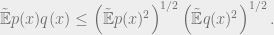
Fact: pseudoexpectation Cauchy-Schwarz.
Let $\tilde{\mathbb{E}}$ be a degree $d$ pseudoexpectation on indeterminates $x_1,\ldots,x_n$ . Let $p(x)$ and $q(x)$ be polynomials of degree at most $d/2$ . Then

$\tilde{\mathbb{E}} p(x) q(x) \leq \left ( \tilde{\mathbb{E}} p(x)^2 \right )^{1/2} \left ( \tilde{\mathbb{E}} q(x)^2 \right ) ^{1/2}.$

As a consequence, if $\tilde{\mathbb{E}}$ has degree $dt$ and $t$ is a power of $2$ , by induction

$\tilde{\mathbb{E}} p(x) \leq \left ( \tilde{\mathbb{E}} p(x)^t \right )^{1/t}.$

Proof of pseudoexpectation Cauchy-Schwarz.

For variety, we will do this proof in the language of matrices rather than linear operators. Let $M$ be the matrix indexed by monomials among $x_1,\ldots,x_n$ of degree at most $d$ , with entries $M(x^\alpha, x^\beta) = \tilde{\mathbb E} x^\alpha x^\beta$ . If $p$ is a polynomial of degree at most $d/2$ , we can think of $p$ as a vector indexed by monomials (whose entries are the coefficients of $p$ ) such that $p^\top M q = \tilde{\mathbb{E}} p(x) q(x)$ . Hence,

$\tilde{\mathbb{E}} p(x) q(x) = \langle M^{1/2} p, M^{1/2} q \rangle \leq \|M^{1/2} p\| \|M^{1/2} q\| = \left ( \tilde{\mathbb{E}} p(x)^2 \right ) ^{1/2} \left ( \tilde{\mathbb{E}} q(x)^2 \right ) ^{1/2}.$

QED.

We will want a second, similar fact.

Fact: pseudoexpectation Holder’s.
Let $p$ be a degree $\ell$ sum of squares polynomial, $t \in \mathbb{N}$ , and $\tilde{\mathbb{E}}$ a degree $O(t \ell)$ pseudoexpectation. Then

$\tilde{\mathbb{E}} p(x)^{t-2} \leq \left ( \tilde{\mathbb{E}} p(x)^t \right )^{\tfrac{t-2}{t}}.$

The proof of pseudoexpectation Holder’s is similar to several we have already seen; it can be found as Lemma A.4 in this paper by Barak, Kelner, and Steurer.

Lemma 2: an SoS version of Lemma 1

We are ready to state and prove our SoS version of Lemma 1. The reader is encouraged to compare the statement of Lemma 2 to the alternative version of Lemma 1. The proof will be almost identical to the proof of the alternative version of Lemma 1.

Lemma 2.
Let $X_1,\ldots,X_n \in \mathbb{R}$ . Let $S_1,\ldots,S_k$ be a partition of $[n]$ into $k$ pieces of size $N = n/k$ such that for each $S_i$ , the collection of numbers $\{X_j\}_{j \in S_i}$ obeys the following moment bound:

$\mathbb{E}_{j \sim S_i} |X_j - \mu_i|^t \leq 2 \cdot t^{t/2}$

where $\mu_i$ is the average $\mathbb{E}_{j \sim S_i} X_j$ and $t$ is a power of $2$ in $\mathbb{N}$ . Let $\Delta > 0$ be such that $|\mu_i - \mu_j| \geq \Delta$ for every $i \neq j$ .

Let $w_1,\ldots,w_n$ be indeterminates. Let $\mathcal{A}$ be the following set of equations and inequalities.

$w_i^2 = w_i \text{ for } i \in [n]$
$\sum_{i \in [n]} w_i = N$
$\frac 1 N \sum_{i \in [n]} w_i \cdot (X_i - \mu)^t \leq 2 \cdot t^{t/2}.$

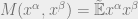
As before $\mu = \mu(w)$ is the polynomial $\tfrac 1 N \sum_{i \in [n]} w_i X_i$ . Thinking of the variables $w_i$ as defining a set $T \subseteq [n]$ via its $0/1$ indicator, let $|T \cap S_j|$ be the formal expression

$|T \cap S_j| = \sum_{i \in S_j} w_i.$

Let $\tilde{\mathbb{E}}$ be a degree $O(t)$ pseudoexpectation which satisfies $\mathcal{A}$ . Then

$\tilde{\mathbb{E}} \left [ \sum_{i \in [k]} \left ( \frac{|T \cap S_i|}{N} \right ) ^2 \right ] \geq 1 - \frac{2^{O(t)} t^{t/2} k^2}{\Delta^t}.$

Proof of Lemma 2.
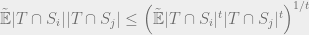
We will endeavor to bound $\tilde{\mathbb{E}} |T \cap S_i| \cdot |T \cap S_j|$ from above for every $i \neq j$ . Since we want to use the degree $t$ polynomials in Fact 2, we get started with

$\tilde{\mathbb{E}} |T \cap S_i| |T \cap S_j| \leq \left ( \tilde{\mathbb{E}} |T \cap S_i|^t |T \cap S_j|^t \right )^{1/t}$

by (repeated) pseudoexpectation Cauchy-Schwarz.

Since $\mu_i = \mathbb{E}_{\ell \sim S_i} X_\ell$ and $\mu_j = \mathbb{E}_{\ell \sim S_j} X_\ell$ are $\Delta$ -separated, i.e. $|\mu_i - \mu_j|^t \geq \Delta^t$ , we also have

$\vdash_t (\mu_i - \mu)^t + (\mu_j - \mu)^t \geq 2^{-t} \left [ (\mu_i - \mu) - (\mu_j - \mu) \right ]^t \geq 2^{-t} \Delta^t$

where the indeterminate is $\mu$ and we have only used the SoS triangle inequality. Hence,

$\tilde{\mathbb{E}} |T \cap S_i|^t |T \cap S_j|^t \leq \tilde{\mathbb{E}} \left [ \frac{(\mu_i - \mu)^t + (\mu_j - \mu)^t }{2^{-t} \Delta^t} |T \cap S_i|^t |T \cap S_j|^t \right ].$

Applying Fact 2 and soundness to the right-hand side, we get

$\tilde{\mathbb{E}} |T \cap S_i|^t |T \cap S_j|^t \leq 2^{O(t)} t^{t/2} \Delta^{-t} \cdot N \cdot \left ( \tilde{\mathbb{E}} |T \cap S_i|^t |T \cap S_j|^{t-1} + \tilde{\mathbb{E}} |T \cap S_i|^{t-1} |T \cap S_j|^t \right ).$

Now using that $\mathcal{A} \vdash_t w_i^2 \leq 1$ and hence $\mathcal{A} \vdash_t |T \cap S_i| \leq N$ and similarly for $|T \cap S_j|$ , we get

$\tilde{\mathbb{E}} |T \cap S_i|^t |T \cap S_j|^t \leq 2^{O(t)} t^{t/2} \Delta^{-t} \cdot N^2 \cdot \tilde{\mathbb{E}} |T \cap S_i|^{t-1} |T \cap S_j|^{t-1}.$

By pseudoexpectation Cauchy-Schwarz

$\tilde{\mathbb{E}} |T \cap S_i|^{t-1} |T \cap S_j|^{t-1} \leq (\tilde{\mathbb{E}} |T \cap S_i|^t |T \cap S_j|^t)^{1/2} (\tilde{\mathbb{E}} |T \cap S_i|^{t-2} |T \cap S_j|^{t-2})^{1/2}$

which, combined with the preceding, rearranges to

$\tilde{\mathbb{E}} |T \cap S_i|^t |T \cap S_j|^t \leq \frac{2^{O(t)} t^t N^4}{\Delta^{2t}} \tilde{\mathbb{E}} |T \cap S_i|^{t-2} |T \cap S_j|^{t-2}.$

By pseudoexpectation Holder’s,

$\tilde{\mathbb{E}} |T \cap S_i|^{t-2} |T \cap S_j|^{t-2} \leq \left ( \tilde{\mathbb{E}} |T \cap S_i|^t |T \cap S_j|^t \right )^{(t-2)/t}.$

All together, we got

$\tilde{\mathbb{E}} |T \cap S_i|^t |T \cap S_j|^t \leq \frac{2^{O(t)} t^t N^4}{\Delta^{2t}} \left ( \tilde{\mathbb{E}} |T \cap S_i|^t |T \cap S_j|^t \right )^{(t-2)/t}.$

Now we no longer have to worry about SoS proofs; we can just cancel the terms on either side of the inequality to get

$\tilde{\mathbb{E}} |T \cap S_i| |T \cap S_j| \leq \left ( \tilde{\mathbb{E}} |T \cap S_i|^t |T \cap S_j|^t \right )^{1/t} \leq \frac{2^{O(t)} t^{t/2} N^2}{\Delta^{t}}.$

Putting this together with

$\tilde{\mathbb{E}} \sum_{ij \in [k]} |T \cap S_i| |T \cap S_j| = \tilde{\mathbb{E}} \left ( \sum_{i \in [n]} w_i \right )^2 = N^2$

finishes the proof. QED.

6 thoughts on “Clustering and Sum of Squares Proofs, Part 3”

samhop says:

December 16, 2017 at 5:07 pm

EDIT: fixed incorrect proof of pseudoexpectation cauchy-schwarz.

Pingback: Clustering and Sum of Squares Proofs, Part 4 | Windows On Theory
Pingback: Clustering and Sum of Squares Proofs, Part 5 | Windows On Theory
Pingback: Clustering and Sum of Squares Proofs, Part 6 | Windows On Theory
Pingback: Sam Hopkins’s 6 part learning via SoS series | Windows On Theory
samhop says:

January 5, 2018 at 5:57 pm

EDIT: fixed incorrect statement of soundness of SoS proofs. Thanks to David Steurer for pointing out the error.

	James Cross on GPT as an “Intelligence…
	Thoughts on AI safet… on AI will change the world, but…
	Anonymous on An alarming trend in K-12 Math…
	Interview about this… on Men in Computer Science
	Interview about this… on The Swiss Army Knife of C…

Clustering and Sum of Squares Proofs, Part 3

The Story So Far

Setting

Remaining obstacles to an SoS version of Lemma 1

Lemma 1 reformulated: maintaining symmetry

Pseudodistributions and duality

Lemma 2: an SoS version of Lemma 1

Published by samhop

6 thoughts on “Clustering and Sum of Squares Proofs, Part 3”

Leave a Reply Cancel reply

The Story So Far

Setting

Remaining obstacles to an SoS version of Lemma 1

Lemma 1 reformulated: maintaining symmetry

Pseudodistributions and duality

Lemma 2: an SoS version of Lemma 1

Share this:

Like this:

Related

Published by samhop

6 thoughts on “Clustering and Sum of Squares Proofs, Part 3”

Leave a Reply Cancel reply