Statistical physics dictionary

I’ve always been curious about the statistical physics approach to problems from computer science. The physics-inspired algorithm survey propagation is the current champion for random 3SAT instances, statistical-physics phase transitions have been suggested as explaining computational difficulty, and statistical physics has even been invoked to explain why deep learning algorithms seem to often converge to useful local minima.

Unfortunately, I have always found the terminology of statistical physics, “spin glasses”, “quenched averages”, “annealing”, “replica symmetry breaking”, “metastable states” etc.. to be rather daunting. I’ve recently decided to start reading up on this, trying to figure out what these terms mean. Some sources I found useful are the fun survey by Cris Moore, the longer one by Zdeborová and Krzakala, the somewhat misnamed survey by Castellani and Cavagna, and the wonderful book by Mezard and Montanari. (So far, I’m still early in the process of looking at these sources. Would appreciate pointers to any others!)

This post is mainly for my own benefit, recording some of my thoughts.
It probably contains many inaccuracies and I’d be grateful if people point them out.

First of all, it seems that statistical physicists are very interested in the following problem: take a random instance of a constraint satisfaction problem, and some number , and sample from the uniform distribution over assignments to the variables that satisfy at least fraction of the constraints. More accurately, they are interested in the distribution where the probability of an assignment is proportional to where is some parameter and is the number of constraints of that violates. However, for an appropriate relation of and , this is more or less the same thing, and so you can pick which one of them is easier to think about or to calculate based on the context.

Physicists call the distribution  the Boltzman distribution, they would call the energy of . Often they would write as where , known as the Hamiltonian, is the general shape of the constraint satisfaction problem, and are the parameters. The internal energy is the typical value of under this distribution, which roughly corresponds to where is the total number of constraints in and (as before) is the fraction of satisfied constraints. The free energy is the sum of the internal energy and the entropy of the Boltzman distribution (the latter multiplied by ).

Why would statistical physicists care about constraint satisfaction problems?

My understanding is that they typically study a system with a large number of particles, and these particles have various forces acting on them. (These forces are local and so each one involves a constant number of particles – just like in constraint satisfaction problems.) These forces push the particles to satisfy the constraints, while temperature (which you can think of as ) pushes the particles to have as much entropy as possible. (It is entropy in a Bayesian sense, as far as I understand; it is not that the particles’ state is sampled from this distribution at any given point in time, it is that our (or Maxwell’s demon’s) knowledge about the state of the particles can be captured by this distribution.) When the system is hot, is close to zero, and the distribution has maximal entropy, when the system is cold, gets closer to infinity, and the fraction of satisfied constraints grows closer to the maximum possible number. Sometimes there is a phase transition where a change in can lead to an change in . (These and factors are with respect to the number of particles , which we think of as tending to infinity; also often we care about higher order phase transition, there the change is in some derivative of ). That is, a small change in the temperature leads to a qualitatively different distribution. This happens for example when a system changes from solid to liquid.

Ideally (or maybe naively), we would think of the state of the system as being just a function of the temperature and not depend on the history of how we got to this temperature, but that’s not always the case. Just like an algorithm can get stuck in a local minima, so can the system get stuck in a so called “metastable state”. In particular, even if we cool the system to absolute zero, its state might not satisfy the global maximum fraction of constraints.

A canonical example of a system stuck in a metastable state is glass. For example, a windowpane at room temperature is in a very different state than a bag of sand in the same temperature, due to the windowpane’s history of first being heated to very high temperatures and then cooled down. In statistical physics lingo the static prediction of the state of the system is the calculation based on its temperature, while a dynamic analysis takes into account the history and the possibility of getting stuck in metastable states for a long time.

Why do statistical physicists care about random constraint satisfaction problems?

So far we can see why statistical physicists would want to understand a constraint satisfaction problem that corresponds to some physical system, but why would they think that is random?

As far as I can tell, there are two reasons for this. First, some physical systems are “disordered” in the sense that when they are produced, the coefficients of the various forces on the particles are random. A canonical example is spin glass. Second, they hope that the insights from studying random CSP’s could potentially be relevant for understanding the actual CSP’s that are not random (e.g., “structured” as opposed to “disordered”) that arise in practice.

In any case, a large body of literature is about computing various quantities of the state of a random CSP at a given temperature, or after following certain dynamics.
For such a quantity , we would want to know the typical value of that is obtained with high probability over . Physicists call this value the “quenched” average (which is obtained by fixing to a typical value). Often it is easier to compute the expectation of over (which is called “annealed average” in physicist-lingo), which of course gives the right answer if the quantity is well concentrated – a property physicists call “self averaging”.

Often if a quantity is not concentrated, the quantity would be concentrated, and so we would want to compute the expectation . The “replica trick” is to use the fact that is the derivative at of the function . So, . (Physicists would usually use instead of , but I already used for the number of variables, which they seem to often call .) Now we can hope to exchange the limit and expectation and write this as . For an integer , it is often the case that we can compute the quantity . The reason is that typically is itself the expectation of some random variable that is parameterized by , and hence would just correspond to taking the expectation of the product of independent copies (or “replicas” in physicist-speak) from these random variables. So, now the hope is that we get some nice analytical expression for , and then simply plug in and hope this gives us the right answer (which surprisingly enough always seems to work in the contexts they care about).

What are the qualitative phase transitions that physicists are interested in?

Let us fix some “typical” and consider the distribution which is uniform over all assignments satisfying an fraction of ‘s constraints (or, essentially equivalently, where the probability of is proportional to ). We will be particularly interested in the second moment matrix of , which is the matrix such that where is sampled from . (Let’s think of as a vector in .)

We can often compute the quantity for every .
By opening up the parenthesis this corresponds to computing for independent from (i.e., “replicas”). (Physicists often think of the related “overlap matrix” which is the matrix where .) This means that we can completely determine the typical spectrum of as a function of the parameters or .

The typical behavior when is small (i.e., the system is “hot”) is that the solutions form one large “cluster” around a particular vector . This is known as the “replica symmetric” phase, since all copies (“replicas”) chosen independently from would have roughly the same behavior, and the matrix above would have on the diagonal and the same value off diagonal.
This means that is close to the rank one matrix . This is for example the case in the “planted” or “hidden” model (related to “Nishimory condition” in physics) if we plant a solution at a sufficiently “easy” regime in terms of the relation between the number of satisfied constraints and the total number of variables. In such a case, it is easy to “read off” the planted solution from the second moment matrix, and it turns out that many algorithms succeed in recovering the solution.

As we cool down the system (or correspondingly, increase ) the distribution breaks into exponentially many clusters. In this case, even if we planted a solution , the second moment matrix will look like the identity matrix (since the centers of the clusters could very well be in isotropic positions). Since there are exponentially many clusters that dominate the distribution, if we sample from this distribution we are likely to fall in any one of them. For this reason we will not see the cluster behavior in static analysis but we will get stuck in the cluster we started with in any dynamic process. This phase is called “1-dRSB” for “one step dynamic replica symmetry breaking” in the physics literature. (The “one step” corresponds to the distribution being simply clustered, as opposed to some hierarchy of sub-clusters within clusters. The “one step” behavior is the expected one for CSP’s as far as I can tell.)

As far as I can tell, the statistical physics predictions would be that this would be the parameter regime where sampling from the distribution would be hard, as well as the regime where recovering an appropriately planted assignment would be hard. However, perhaps in some cases (e.g., in those arising from deep learning?) we are happy with anyone of those clusters.

If we cool the system more then one or few clusters will dominate the distribution (this is known as condensation), in which case we get to the “static replica symmetry breaking” phase where the second moment matrix changes and has rank corresponding to roughly the number of clusters. If we then continue cooling the system more then the static distribution will be the global optimum (the planted assignment if we had one), though dynamically we’ll probably be still stuck in one of those exponentially many clusters.

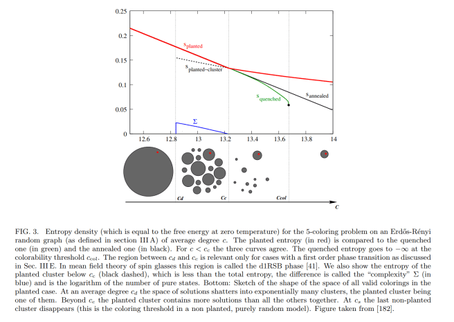
The figure below from Zdeborová and Krzakala illustrates these transitions for the 5 coloring constraint satisfaction problem (the red dot is the planted solution). This figure is as a function of the degree of the graph $c$, whereas increasing the degree can be thought of as making the system “colder” (as we are adding more constraints the system needs to satisfy).

What about algorithms?

I hope to read more to understand belief propagation, survey propagation, various Markov Chain sampling algorithms, and how they might or might not relate to the sum of squares algorithm and other convex programs. Will update when I do.

Update 10/6/2021: Fixed some errors, also see this lecture on statistical physics and inference, and these two posts (part I, part II) on the replica method, written by Blake Bordelon and Haozhe Shan, together with  Abdul Canatar,  Cengiz Pehlevan and me.