Discrepancy theory seeks to understand how well a continuous object can be approximated by a discrete one, with respect to some measure of uniformity. For instance, a celebrated result due to Joel Spencer says that given any set family ![{S_1,\ldots,S_n\subset [n]}](https://s0.wp.com/latex.php?latex=%7BS_1%2C%5Cldots%2CS_n%5Csubset+%5Bn%5D%7D&bg=eeeeee&fg=000000&s=0&c=20201002) , it is possible to color the elements of
, it is possible to color the elements of ![{[n]}](https://s0.wp.com/latex.php?latex=%7B%5Bn%5D%7D&bg=eeeeee&fg=000000&s=0&c=20201002) Red and Blue in a manner that:
Red and Blue in a manner that:
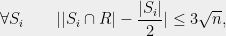
where ![{R\subset [n]}](https://s0.wp.com/latex.php?latex=%7BR%5Csubset+%5Bn%5D%7D&bg=eeeeee&fg=000000&s=0&c=20201002) denotes the set of red elements. In other words, it is possible to partition into two subsets so that this partition is very close to balanced on each one of the test sets
denotes the set of red elements. In other words, it is possible to partition into two subsets so that this partition is very close to balanced on each one of the test sets  . Note that a ‘continuous’ partition which splits each element exactly in half will be exactly balanced on each ; the content of Spencer’s theorem is that we can get very close to this ideal situation with an actual, discrete partition which respects the wholeness of each element.
Spencer’s theorem and its variants have had applications in approximation algorithms, numerical integration, and many other areas. In this post I will describe a new discrepancy theorem due to Adam Marcus, Dan Spielman, and myself, which also seems to have many applications. The theorem is about `uniformly’ partitioning sets of vectors in  and says the following:
Theorem 1 (implied by Corollary 1.3 in Interlacing Families II)
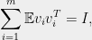
Given vectors  satisfying
  and
and
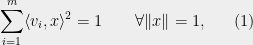
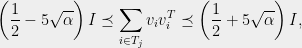
there exists a partition ![{T_1\cup T_2=[m]}](https://s0.wp.com/latex.php?latex=%7BT_1%5Ccup+T_2%3D%5Bm%5D%7D&bg=eeeeee&fg=000000&s=0&c=20201002) satisfying
satisfying
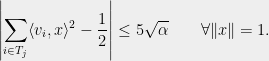
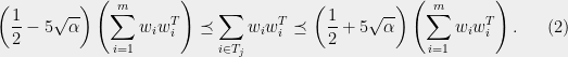
Thus, instead of being nearly balanced with respect to a finite set family as in Spencer’s setting, we require our partition of  to be nearly balanced with respect to the infinite set of test vectors
  . In this context, `nearly balanced’ means that about half of the quadratic form (`energy’) of the
  in direction
  comes from
  (and the rest, which must also be about half, comes from
  ). We will henceforth refer to the maximum deviation from perfect balance (i.e.,
  ) over all as the discrepancy of a partition. Note that every partition has discrepancy at most , so the guarantee of the theorem is nontrivial whenever
  .
.
This type of theorem was conjectured to hold by Nik Weaver, with any constant strictly less than  (independent of
  and
and  ) in place of
  . The reason he was interested in it is that he showed it implies a positive solution to the so-called Kadison-Singer (KS) problem, a central question in operator theory which had been open since 1959. KS was itself motivated by a basic question about the mathematical foundations of quantum mechanics — check out the blog soulphysics for a discussion of its physical significance. If you want to know exactly what the statement of KS is and how it can be reduced to finite-dimensional vector discrepancy statements similar to Theorem 1, I highly recommend the accessible and self-contained survey article written recently by Nick Harvey.
In the rest of the post I will try to demystify what Theorem 1 is about, say a bit about its proof, and describe a simple application to graph theory.
What the Theorem Says
Let’s examine how restrictive the hypotheses of Theorem 1 are. To see that some bound on the norms of the  is necessary for the conclusion of the theorem to hold, consider an example where one vector has large norm, say
  In any partition of , one of the sets, say , will contain
  . If we now examine the quadratic form in the direction
  , we see that

so this partition has discrepancy at least  . The problem is that by itself accounts for significantly more than half of the quadratic form in direction , and there is no way to get closer to half without splitting the vector.
Another instructive example is the one-dimensional instance  , with
  for all
  and odd. Here, the larger side of any partition must have
  leading to a discrepancy of at least
  .
.
In general, the above examples show that the presence of large vectors is an obstruction to the existence of a low discrepancy partition. Theorem 1 shows that this is the only obstruction, and if all the vectors have sufficiently small norm then an appropriately low discrepancy partition must exist. It is worth mentioning that by a more sophisticated example than the ones above, Weaver has shown that the  dependence in Theorem 1 cannot be improved.
Let us now consider the `isotropy’ condition (1). This may seem like a very strong requirement at first, but it is in fact best viewed as a normalization condition. To see why, let us first write the theorem using matrix notation. It says that given vectors 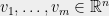 with
with  and
and

there is a partition satisfying
where  means that

or equivalently that  is positive semidefinite.
Now suppose I am given some arbitrary vectors  , which are not necessarily isotropic. Assume that the span of the
  is (otherwise, change the basis and write them as vectors in some lower dimensional
  ). This implies that the positive semidefinite matrix
  is invertible, and therefore has a negative square root
  . Now consider the `normalized’ vectors

and observe that

so these vectors are isotropic. The normalized vectors have norms

To better grasp what these norms mean, we can write:

Thus, the norms  measure the maximum fraction of the quadratic form of
  that a single vector can be responsible for — exactly the critical quantity in the example at the beginning of this section.
These numbers are sometimes called `leverage scores’ in numerical linear algebra and statistics. As long as the leverage scores are bounded by  , we can apply Theorem 1 to
  to obtain a partition satisfying
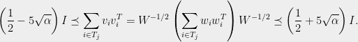
We now appeal to the fact that iff  , for any invertible
  (this amounts to a simple change of variables similar to what we did in (*)). Multiplying by
  on both sides, we find that the partition
  guaranteed by Theorem 1 satisfies:
Thus, we have the following restatement of Theorem 1:
Theorem 2 Given any vectors , there is a partition such that (2) holds with  .
.
Note that we have used the pseudoinverse instead of the usual inverse to handle the case where the vectors do not span .
For those who do not like to think about sums of rank one matrices (I know you’re out there), Theorem 2 may be restated very concretely as:
Theorem 3 Any matrix  whose rows
  have leverage scores
  bounded by can be partitioned into two row submatrices
  and
and  so that for all

The reason this theorem is powerful is that lots of diverse objects can be encoded as quadratic forms of matrices. We will see one such application later in the post.
Matrix Chernoff Bounds and Interlacing Polynomials
Let me quickly say a bit about the proof of Theorem 1. One reasonable way to try to find a good partition is randomly, and indeed this strategy is successful to a certain extent. The tool that we use to analyze a random partition is the so-called ‘Matrix Chernoff Bound’, developed and refined by Pisier, Lust-Piquard, Rudelson, Ahlswede-Winter, Tropp, and others. The variant that is most convenient for our application is the following:
Theorem 4 (Theorem 4.1 in Tropp)
Given symmetric matrices  and independent random Bernoulli signs
  , we have
![\displaystyle \mathbb{P}\left[ \left\|\sum_{i=1}^m \epsilon_i A_i\right\|\ge t\right]\leq 2n\cdot \exp\left(-\frac{t^2}{2 \|\sum_{i=1}^m A_i^2\|}\right).](https://s0.wp.com/latex.php?latex=%5Cdisplaystyle+%5Cmathbb%7BP%7D%5Cleft%5B+%5Cleft%5C%7C%5Csum_%7Bi%3D1%7D%5Em+%5Cepsilon_i+A_i%5Cright%5C%7C%5Cge+t%5Cright%5D%5Cleq+2n%5Ccdot+%5Cexp%5Cleft%28-%5Cfrac%7Bt%5E2%7D%7B2+%5C%7C%5Csum_%7Bi%3D1%7D%5Em+A_i%5E2%5C%7C%7D%5Cright%29.&bg=eeeeee&fg=000000&s=0&c=20201002)
Applying the theorem to  and taking
  yields Theorem 1 with a discrepancy of
  , which is nontrivial when
  . This bound is interesting and useful in some settings, but it is not sufficient to prove the Kadison-Singer conjecture (which requires a uniform bound as
  ), or for the application in the next section. It may be seen as analogous to the discrepancy of
  achieved by a random coloring of a set family , which is easily analyzed using the usual Chernoff bound and a union bound.
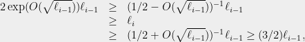
In order to remove the logarithmic factor and obtain Theorem 1, we prove the following stronger but less general inequality, which controls the deviation of a sum of independent rank-one matrices at a constant rather than logarithmic scale, but only with nonzero (rather than high) probability:
Theorem 5 (Theorem 1.2 in Interlacing Families II)
If  and
and  are independent random vectors in
  with finite support such that
and  for all , then
![\displaystyle \mathbb{P}\left[ \left\|{\sum_{i=1}^m v_i v_i^{T}}\right\| \leq (1 + \sqrt{\alpha})^2 \right] > 0](https://s0.wp.com/latex.php?latex=%5Cdisplaystyle+%5Cmathbb%7BP%7D%5Cleft%5B+%5Cleft%5C%7C%7B%5Csum_%7Bi%3D1%7D%5Em+v_i+v_i%5E%7BT%7D%7D%5Cright%5C%7C+%5Cleq+%281+%2B+%5Csqrt%7B%5Calpha%7D%29%5E2+%5Cright%5D+%3E+0+&bg=eeeeee&fg=000000&s=0&c=20201002)
The conclusion of the theorem is equivalent to the following existence statement: there is a point  in the probability space implicitly defined by the ‘s such that

To prove the theorem, we begin by considering for every  we the univariate polynomial
 := \det\left(xI - \sum_{i\le m}v_i(\omega)v_i(\omega)^T\right).](https://s0.wp.com/latex.php?latex=%5Cdisplaystyle+P%5B%5Comega%5D%28x%29+%3A%3D+%5Cdet%5Cleft%28xI+-+%5Csum_%7Bi%5Cle+m%7Dv_i%28%5Comega%29v_i%28%5Comega%29%5ET%5Cright%29.&bg=eeeeee&fg=000000&s=0&c=20201002)
The roots of ![{P[\omega]}](https://s0.wp.com/latex.php?latex=%7BP%5B%5Comega%5D%7D&bg=eeeeee&fg=000000&s=0&c=20201002) are real since it is the characteristic polynomial of a symmetric matrix, and in particular the largest root is equal to the spectral norm of
are real since it is the characteristic polynomial of a symmetric matrix, and in particular the largest root is equal to the spectral norm of  .
.
The proof now proceeds in two steps. First, we show that there must exist an such that
![\displaystyle \lambda_{max}(P[\omega])\le \lambda_{max}(\mathbb{E} P), \ \ \ \ \ (3)](https://s0.wp.com/latex.php?latex=%5Cdisplaystyle+%5Clambda_%7Bmax%7D%28P%5B%5Comega%5D%29%5Cle+%5Clambda_%7Bmax%7D%28%5Cmathbb%7BE%7D+P%29%2C+%5C+%5C+%5C+%5C+%5C+%283%29&bg=eeeeee&fg=000000&s=0&c=20201002)
where  denotes the largest root of a polynomial. This type of statement may be seen as a generalization of the probabilistic method to polynomial-valued random variables, and was introduced in the paper Interlacing Families I, where we used it to show the existence of bipartite Ramanujan graphs of every degree by proving a conjecture of Bilu and Linial. Note that (3) does not hold for general polynomial-valued random variables — in general, the roots of a sum of polynomials do not have much to do with the roots of the individual polynomials. The reason it holds in this particular case is that the are generated by sums of rank-one matrices, which by Cauchy’s theorem produce interlacing characteristic polynomials and form what we call an `interlacing family’.
The second step is to upper bound the roots of the expected polynomial  It turns out that the right way to do this is to write
  as a linear transformation of a certain
  variate polynomial
  , and show that
  does not have any roots in a certain region of
  . This is achieved by a new multivariate generalization of the `barrier function’ argument used in this paper to construct spectral sparsifiers of graphs. The multivariate barrier argument relies heavily on the theory of real stable polynomials, which are a multivariate generalization of real-rooted polynomials.
See this post for an elementary and self-contained demonstration of the method, in which it is used to solve a slightly easier problem. Rather than give any further details, I encourage you to read the paper. The proof is not difficult to follow, and from what I have heard quite `readable’.
Partitioning a Graph into Sparsifiers
One very fruitful setting in which to apply Theorem 2 is that of Laplacian matrices of graphs. Recall that for an undirected graph  on vertices, the Laplacian is the
  symmetric matrix defined by:

where  is the incidence vector of the edge
  . The Laplacian quadratic form
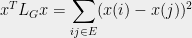
encodes a lot of useful information about a graph. For instance, it is easy to check that given any cut  , the quadratic form
  of the indicator vector
  is equal to the number of edges between
  and
and  . Thus, the values of
  completely determine the cut structure of
  . (We mention in passing that the extremizers of the quadratic form are eigenvalues and are related to various other properties of — this is the subject of spectral graph theory.)
Now consider  , the complete graph on vertices, which has Laplacian
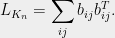
An elementary calculation reveals that the leverage scores in this graph are all very small:
This is a good time to mention that the leverage scores of the incidence vectors  in any graph have a natural interpretation — they are simply the effective resistances of the edges when the graph is viewed as an electrical network (this happens because inverting
  is equivalent to computing an electrical flow, and the quantity
  is equal to the energy dissipated by the flow.) In any case, for the complete graph all of the edges have effective resistances equal to
  , so we may apply Theorem 2 with
  to conclude that there is a partition of the edges into two sets, and , each satisfying

Now observe that each sum over  is the Laplacian
  of a subgraph
  of
of  . By recalling the connection to cuts, this implies that
  can be partitioned into two subgraphs,
  and
and  , each of which approximates its cuts upto a
  factor.
This seems like a cute result, but we can go a lot further. As long as the effective resistances of edges in and sufficiently small, we can apply Theorem 2 again to each of them to obtain four subgraphs. And then again to obtain eight subgraphs, and so on.
How long can we keep doing this? The answer depends on how fast the effective resistances grow as we keep partitioning the graph. The following simple calculation reveals that they grow geometrically at a favorable rate. Initially, all of the effective resistances are equal to  . After one partition, the maximum effective resistance of an edge in is at most

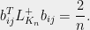
In general, after levels of partitioning, we have the inequalities:
as long as  is bounded by some sufficiently small absolute constant
  . Applying these inequalities iteratively we find that after
  levels:
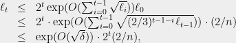
and the inequalities are valid as long as we maintain that  . Taking binary logs, we find that these conditions are satisfied as long as

which means we can continue the recursion for

levels. This yields a partition of into  subgraphs, each of which is an
  -factor spectral approximation of
  , in the sense of (4). This latter approximation property implies that each of the graphs must have constant degree (by considering that the degree cuts must approximate those of ) and constant spectral gap; thus we have shown that can be partitioned into constant degree expander graphs.
The real punchline, however, is that we did not use anything special about the structure of other than the fact that its effective resistances are bounded by  . In fact, the above proof works exactly the same way on any graph on vertices with edges, whose effective resistances are bounded by
  — for such a graph, the same calculations reveal that we can recursively partition the graph for
  levels, while maintaining a constant factor approximation! Note that the total effective resistance of any unweighted graph on vertices is
  , so the boundedness condition is just saying that every effective resistance is at most a constant times the average over all edges.
For instance, the effective resistances of all edges in the hypercube  on
on  vertices are very close to
  . Thus, repeatedly applying Theorem 2 implies that it can be partitioned into
  constant degree subgraphs, each of which is an
  approximation of
  . In fact, this type of conclusion holds for any edge-transitive graph, in which symmetry implies that each edge has exactly the same effective resistance.
The above result may be seen as a generalization of the theorem of Frieze and Molloy, which says that upto a certain extent any sufficiently good expander graph may be partitioned into sparser expander graphs. It may also seen as an unweighted version of the spectral sparsification theorem of Batson, Spielman, and myself, which says that every graph has a weighted -factor spectral approximation with edges. The recursive partitioning argument that we have used is quite natural and appears to have been observed a number of times in various contexts; see for instance this paper of Rudelson, as well as the very recent work of Harvey and Olver.
Conclusion and Open Questions
Theorem 1 essentially shows that under the mildest possible conditions, a quadratic form / sum of outer products can be `split in two’ while preserving its spectral properties. Since graphs can be encoded as quadratic forms / outer products, the theorem implies that they also can be split into two while preserving some properties. However, a lot of other objects can also be encoded this way. For instance, applying Theorem 1 to a submatrix of a Discrete Fourier Transform (it also holds over  ) or Hadamard matrix yields a strengthening of the `uncertainty principle’ for Fourier matrices, which says that a signal cannot be localized both in the time domain and the frequency domain; see this paper of Casazza and Weber for details. This strengthening has implications in signal processing, and its infinite dimensional analogue is useful in analytic number theory. For a thorough survey of the consequences of the Kadison-Singer conjecture and Theorem 1 in many diverse areas, check out this survey.
To conclude, let me point out that the current proof of Theorem 1 is not algorithmic, since it involves reasoning about polynomials which are in general  -hard to compute. Finding a polynomial-time algorithm which delivers the low-discrepancy partition promised by the theorem is likely to yield further insights into the techniques used to prove it as well as more connections to other areas — just as the beautiful work of Moser-Tardos, Bansal, and Lovett-Meka has done for the Lovasz Local Lemma and Spencer’s theorem. It would also be nice to see if the methods used here can be used to recover known results in discrepancy theory, such as Spencer’s theorem itself.
Acknowledgments
Thanks to Nick Harvey, Daniel Spielman, and Nisheeth Vishnoi for helpful suggestions, comments, and corrections during the preparation of this post.

Wonderful result! It is nice how a classical question with analysis is related to discrapancy-theory, partitioning graphs into expanders and related questions in discrete mathematics and TOC. Of course the interlacing polynomial method looks very powerful. A well known discrepancy problem which is still open is Komlos’ conjecture.
Great result, and very nicely explained! BY the way, in the first paragraph, what is the role of m? Surely it fails for m=2^n?
Thanks for the correction! It have changed it to S_1…S_n\subset [n]. (The bound for S_1…S_m is \sqrt{nlog(m/n)}, but I chose to go with this for simplicity.)