Fun and Games with Sums of Squares

This blog post is an introduction to the “Sum of Squares” (SOS) algorithm from my biased perspective. This post is rather long – I apologize. You might prefer to view/print it in pdf format. If you’d rather “see the movie”, I’ll be giving a TCS+ seminar about this topic on Wednesday, February 26th 1pm EST. If you prefer the live version, I’ll be giving a summer course in Stockholm from June 30 till July 4th. I’ve been told that there are worse places to be in than Stockholm in June, and there are definitely worse things to do than taking a course on analysis of Boolean functions from Ryan O’Donnell, which will also be part of the same summer school.

This post starts with an 1888 existential proof by Hilbert, given a constructive version by Motzkin in 1965. We will then go through proof complexity and semidefinite programming to describe the SOS algorithm and how it can be analyzed. Most of this is based on my recent paper with Kelner and Steuer and a (yet unpublished) followup work of ours, but we’ll also discuss notions that can be found in our previous work with Brandao, Harrow and Zhou. While our original motivation to study this algorithm came from the Unique Games Conjecture, our methods turn out to be useful to problems from other domains as well. In particular, we will see an application for the Sparse Coding problem (also known as dictionary learning) that arises in machine learning, computer vision and image processing, and computational neuroscience. In fact, we will close a full circle as we will see how polynomials related to Motzkin’s end up playing a role in our analysis of this algorithm.

I am still a novice myself in this area, and so this post is likely to contain inaccuracies, misattributions, and just plain misunderstandings. Comments are welcome! For deeper coverage of this topic, see Pablo Parrilo’s lecture notes, and Monique Laurent’s monograph. A great accessible introduction from a somewhat different perspective is given in Amir Ali Ahmadi’s blog posts (part I and part II). In addition to the optimization applications discussed here, Amir mentions that “in dynamics and control, SOS optimization has enabled a paradigm shift from classical linear control to … nonlinear controllers that are provably safer, more agile, and more robust” and that SOS has been used in “areas as diverse as quantum information theory, robotics, geometric theorem proving, formal verification, derivative pricing, stochastic optimization, and game theory”.

1. Sum of squares and the Positivstellensatz

One of the tedious exercises in high school mathematics involves finding the minimal value of a polynomial such as

To solve this, we were taught to go over all critical points (where the derivative vanishes) and check their values, so eventually we get a picture like this

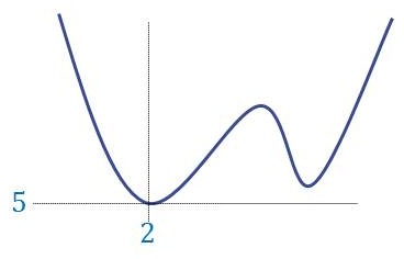
and can deduce that the minimum is achieved at the point .

As theoretical Computer Scientists, we can make this feeling of tedium precise— this method involves exhaustive search over all local optima and hence can take time for an -variate polynomial, even if it is only of degree . Unfortunately, in general, we do not know of a better way. Indeed, in practice people use generalizations of the high school method such as Gradient Descent to solve such problems, and unsurprisingly often these algorithms do not return the global minimum but get stuck at some local optima. In fact, we know one cannot do better in the worst case, as one can easily transform an -variable 3SAT formula into an -variable degree- polynomial which will have as its global minimum if and only if is satisfiable. (It is easy to come up with a degree polynomial such that for every , equals the number of clauses satisfied by , while the second term is strictly positive for any . See also Ahmadi’s blog post for a reduction to a degree polynomial.)

However, some times there is a nicer, more global way to argue about the extremal points of polynomials. For example, one can see that the minimum of the polynomial in (1) is equal to by writing it as

using the simple (but deep!) fact that a square of a number is never negative.

Bruce Reznick paraphrased Jane Austen to say

It is a truth universally acknowledged, that a mathematical object whose orderings are non-negative must be in want of a representation as a sum of squares.

Despite this saying, the 3SAT example above implies that (assuming NPcoNP) there exists a non-negative polynomial that is not equal to a sum of squares (SOS) of other polynomials, as otherwise we could have had a short proof of unsatisfiability for every 3SAT formula. However proving the existence of such a polynomial unconditionally is not so trivial. Hilbert first gave a non-constructive proof in 1888, and it took almost 80 years until Motzkin gave an explicit example: the Arithmetic-Mean Geometric-Mean (AMGM) inequality implies that the polynomial

is always non-negative since the last term is the geometric mean of , , and , but it turns out that it does not equal a sum of squares. (See Reznick’s or Schmüdgen’s surveys for the proof and more on the history of this problem.)

However, we cam still prove Motzkin’s polynomial is non-negative via a simple and short “SOS proof” since it is the sum of squares of four rational functions:

Already Hilbert was aware of this notion of SOS proofs, and asked as his 17th problem whether we can always certify the non-negativity of any polynomial by such a proof. Through works of Artin (1927), Krivine (1964), and Stengle (1974), we know the answer is a resounding yes!. These results, which serve as the foundation of real algebraic geometry, are known as the Positivstellensatz and hold for even more general polynomial equalities and inequalities. In particular, given some polynomials , the set of equations

is unsatisfiable if and only if this can be certified by finding polynomials and a sum of squares polynomial such that

(The Positivstellensatz applies to polynomials inequalities as well, but in the context of optimization, one can always transform an inequality into the equality by introducing an auxiliary variable . Even without using inequalities, the Positivstellensatz fundamentally relies on the fact that the real numbers, as opposed to complex numbers, are well ordered.)

2. Proof systems and algorithms

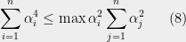
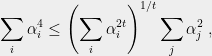
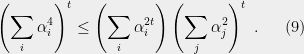
As Theoretical Computer Scientists, we typically try to make qualitative questions into quantitative ones, and indeed in 1999 Gregoriev and Vorobjov defined the Positivstellensatz proof complexity of a set of equations as the minimal degree needed for the polynomials and in (4). Note that a degree SOS proof can always be written down using coefficients, and hence the 3SAT example suggests that at least some equations require a large (i.e., ) degree, and such a result was indeed shown by Grigoriev in 2001.

Bounds on the degree turn out to be very important for optimization as well. Several researchers, including N. Shor, Y. Nesterov, P. Parrilo, and J. Lasserre, realized independently that it is possible to search for a degree SOS proof in time . This follows from a correspondence between polynomials that are sums of squares and positive semidefinite (p.s.d.) matrices; combined with the fact that the latter convex set has an efficient separation oracle, and hence can be efficiently optimized over. (This is known as semidefinite programming.) Indeed, for any -variable degree- polynomial we can define an matrix such that for every , . (As written this assumes is a homogenous polynomial, but this can be suitably generalized to the non-homogenous case as well.) By definition, the matrix is p.s.d. if and only if it equals for some vectors . Therefore one can see that if is p.s.d. then each one of those ‘s defines a degree polynomial such that for every . The other direction works in a similar way.

So, we can efficiently certify the unsatisfiability of a set of polynomial equations if it has a low degree SOS proof. But under what conditions will it have such a proof? and what about finding solutions for satisfiable polynomial equations?

Progress on these questions has been quite slow. For computational problems of interest, degree upper and lower bounds have both been very hard to come by. We essentially knew only one degree lower bound— Gregoriev’s result mentioned above (later rediscovered by Schoenebeck and expanded upon by Tulsiani). As for upper bounds, until very recently we essentially had none, in the sense of having no significant algorithmic results using the SOS algorithm that did not already follow from weaker algorithms. However, some recent results, including the quasipolynomial time quantum separability algorithm of Brandao, Christiandl and Yard, and our results on solving “hard” unique games instances, gave some signs that the SOS framework does have the potential to solve problems beyond the reach of other techniques. In a very recent work with Kelner and Steurer, we show a general way to exploit the power of SOS, which I will now describe.

3. Pseudoexpectations and Combining algorithms

Our approach for using SOS to solve computational problems is based on the following wise proverb

It is easier to solve a problem if you already have a solution.

Specifically, fix the set of polynomial equations (3). A combining algorithm is an algorithm that takes as input a (multi) set of solutions for (3), and outputs a single solution . Based on the proverb above, I guess most readers of this blog would be able to come up with such an algorithm. Now, to make things more challenging, imagine that does not get represented as a list of all its elements (which, after all, could be exponentially large), but rather only gets some low order statistics of . That is, for some smallish (say or ), gets a vector such that for every , (where we identify with the distribution over its elements). This is indeed a harder task, but it still seems much easier than solving the problem from scratch. Surprisingly, it turns out that you can often reduce solving the equations to constructing such a combining algorithm. Our approach works as follows— given a combining algorithm , instead of giving it moments of an actual distribution over solutions (which of course we don’t have), we feed it with a “fake moment” vector . If we’re lucky, won’t notice the difference and will still output a good solution .

How do we construct those “fake moments”? and when will we be lucky? Those “fake moments” are more formally known as pseudoexpectations, and can be found using a semidefinite program which is the dual to the SOS program. In particular, they will obey some of the consistency properties of actual moments, most importantly that for every degree polynomial , if we combine the fake moments given by linearly to compute the presumed value of then it will be non-negative. Those properties imply that if we have a proof that works as combining algorithm, and that proof can be encapsulated in the SOS framework with not too high a degree, then that proof in fact shows that will still output a good solution even when it is fed the fake moments.

4. Machine learning application: the sparse coding problem

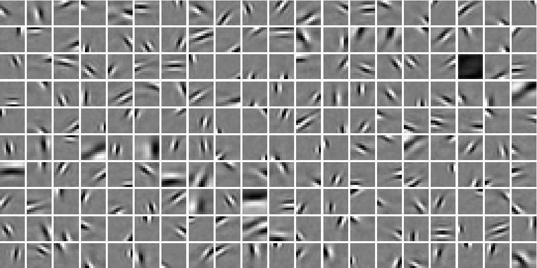
To make things more concrete, we now sketch an example taken from an upcoming paper with Kelner and Steurer. One can see other examples in our original paper. One of the challenging tasks for machine learning is to find good representations for data. For example, representing a picture as a bitmap of pixel works great for projecting it on a screen, but not is not as well suited for trying to decide if it’s a picture of a cat or a dog. Finding the “right” representation for, say, images, is often a first task not just in learning applications, but also for other tasks such as edge detection, image denoising, image completion and more. Sparsity is one way to capture “rightness” of representation. For example, it is often the case that the data is sparse when represented in the “right” linear basis (such as the Fourier or wavelet bases). Olshausen and Field (1997) argued that this may be the way that images are represented by in visual cortex, and they used a heuristic alternating-minimization based algorithm to recover the following basis (also known as a dictionary) for natural images.

But of course as theorists we are not satisfied with a heuristic that works fast and achieves good results. We want a slower algorithm with worse performance that we can prove something about. This is where Sum of Squares comes to the rescue. (At least on some of the counts: it is definitely slower, and we can prove something about it; however “unfortunately” beyond just amenability to analysis there is an (unverified) chance that it actually outperforms the heuristics on some instances, since at least in principle it can avoid getting stuck in local minima.) Recently there have been several works giving rigorous guarantees for sparse coding (e.g., [SWW12 , AGM13, AAJNT13]) but all of them require the representations to be “super-sparse”- have less than significant non-zero coordinates. (There are some works handling the denser case such as [ FJK96, GVX13 , ABGM14] , but they make rather strong assumptions on the dictionary and/or distribution of samples.) In our new work, we use the SOS algorithm to recover the dictionary even as long as the number of nonzero coefficients is less than for some sufficiently small constant . (For these parameters our algorithms takes quasipolynomial time; it takes polynomial time if the number of nonzero coefficients is at most for an arbitrarily small .)

We now sketch the ideas behind the solution. For simplicity of notation, lets assume that the “right basis” is in fact an orthonormal basis , and that we obtain examples of the form , where the ‘s are independently and identically distributed random variables with and for some . Like the works [AGM13, AAJNT13], our methods apply to much more general settings, including non-independent ‘s and overcomplete dictionaries, but this is a good case to keep in mind.

We focus on the task of approximately recovering a single basis vector: once you have such a subroutine, recovering all vectors is not that hard. We do so in three steps:

1. Using the examples observed, we construct a system of polynomial equations. We argue that any solution to is a good solution for us (namely close to one of the basis vectors).

   More concretely, we will find some polynomial whose projection on the sphere looks somewhat like this

   

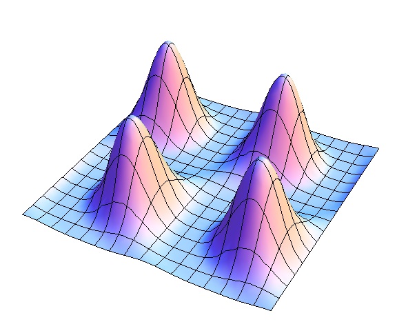
   and whose maximum points correspond to the unknown vectors of our dictionary.

2. On its own, phrasing the question as a polynomial system is not necessarily helpful, since is not convex, and so in general we don’t know how to solve it. However, we do show how to solve the easier problem of coming up with a combining algorithm , that given the low order moments of a distribution over solutions of , manages to recover a single solution.

3. We then verify that all our arguments in Steps 1 and 2 can be encapsulated in the SOS proof system with a low degree, and hence will still work even when fed “fake moments”, thus establishing the result.

We now describe how to implement those three steps.

Step 1: The system of equations. Given examples each one of the form , we construct the polynomial , and consider the equations defined as follows:

(As mentioned before, we can always translate the inequality into an equality by adding an auxiliary variable.)

As grows, converges to the polynomial

It suffices to take to get good enough convergence for our purposes, and so we will just assume that is equal to (5). Opening the parenthesis, and using the fact that and , we see that

which equals

since the ‘s are an orthonormal basis.

Note that for all , and hence the system is feasible. Moreover, if and then

which for equals (using the fact that the ‘s are an orthonormal basis), and this means
which means that

for some .

Step 2: Combining algorithm. I will describe a particularly simple combining algorithm that will involve moments up to logarithmic order, and hence result in a quasipolynomial time algorithm. Under some conditions (namely ) we are able to give a polynomial-time algorithm.

The combining algorithm gets access to a distribution over solutions of , and needs to output a single solution. We do so by choosing a set of random gaussian vectors for , and consider the matrix defined as

where . We output the top eigenvector of .

We claim that with probability , this vector will be highly correlated with one of the ‘s. To see this, note that every element in the support of is very close to one of the ‘s. In particular, there is an such that is close to with probability at least . We can assume without loss of generality, and so is a convex combination of two distributions and such that every element in the support of is close to .

Note that for any unit vector , for a standard Gaussian and hence . Now let us condition on the event that all of the vectors satisfy ; this will happen with probability. This would mean that is roughly for that is close to , while it has a much lower value for ‘s that are not close to it. Thus, almost all the weight in (7) is on the ‘s close to , meaning that is roughly equal to a constant times , and in particular its top eigenvector will be close to .

Step 3: Lifting to pseudoexpectations. Step~3 is in some sense the heart of the proof, moving from a combining algorithm, that requires an actual distribution (which we don’t have), to a rounding algorithm, that only needs a pseudo-distribution (which we can find using semidefinite programming). However, it is also the most tedious, since it involves going over the steps of the proof one by one, verifying that each one only used SOS arguments. However, occasionally “lifting” the proofs for pseudoexpectations requires more care. Rather than giving the full proof here, we show just one example of how we deal with one of those more subtle cases.

Recall that while deriving (6), we used the following simple inequality:

(substituting for ). One challenge in lifting this inequality to pseudo-expectations is that the operation is not a low degree polynomial. Since the norm can be approximated by the norm for large , it turns out it suffices to prove the statement

for some large . Of course to make this a polynomial statement, we need to raise this to the power and get

(9) becomes non-trivial to prove in SOS for so let us focus on the case. The LHS has the form

The RHS has the form

Fixing some particular , and dividing both sides by we see we need to show that

(10) follows from

but this is just our old friend the AMGM inequality . We might worry that this is very related to Motzkin’s polynomial, whose claim to fame is exactly the fact that despite being non-negative, it is not a sum of squares. There are two answers to this concern. The first one is that we don’t care, since Motzkin’s polynomial does have a low degree SOS proof (using its representations as a sum of squares of rational functions) and this is good enough for us to show that it holds for pseudo-expectations as well. The second one is that, at least in my experience, if you stare at (11) long enough, then eventually you get tired of staring, look up and realize you are in a workshop on semidefinite programming, where you can easily find an expert or two that will show you why the RHS minus the LHS is actually a sum of squares. ((Apparently, this was already proven by Hurwitz in 1891, see equation (1.6)
here.) Thus (11) holds if the ‘s come from a pseudo-expectation, which is what we wanted to prove. (Going over the proof, one can see that it can extend into a much more general settings of both the dictionary and the distribution.)

Conclusion

While until recently we had very little tools to take advantage of the SOS algorithm (at least in the sense of having rigorous analysis), we now have some indications that, when applied to the right problems it can be a powerful tool, that may may be able to goals that resisted previous attempts. We have seen some examples of this phenomenon, but I hope (and believe) the best is yet to come, and am looking forward to seeing how this research area develops in the near future.

Acknowledgements. Many thanks to David Steurer for great suggestions, corrections, and insights that greatly improved this blog post, as well as for patiently explaining to me for the nth time the difference between the Positivstellensatz and Nullstellensatz. Thanks to Amir Ali Ahmadi, Jon Kelner, and Pablo Parrilo for showing me the SOS proof for (11) in the ICERM workshop on semidefinite programming and graph partitioning. Thanks to Amir for also pointing out an error in my previous reduction from 3SAT.