[This is the sequel to Jelani’s previous post on chaining method; for more, see the post STOC workshop on this topic –Boaz]
1. A case study: (sub)gaussian processes
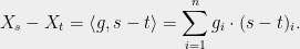
To give an introduction to chaining, I will focus our attention on a concrete scenario. Suppose we have a bounded (but possibly infinite) collection of vectors  . Furthermore, let
  be a random vector with its entries being independent, mean zero, and unit variance gaussians. We will consider the collection of variables
  with
with  defined as
  . In what follows, we will only ever use one property of these :

This provides us with some understanding of the dependency structure of the . In particular, if  are close in
  , then it’s very likely that the random variables
  and are also close.
Why does this property hold? Well,
We then use the property that adding independent gaussians yields a gaussian in which the variances add. If you haven’t seen that fact before, it follows easily from looking at the Fourier transform of the gaussian pdf. Adding independent random variables convolves their pdfs, which pointwise multiplies their Fourier transforms. Since the Fourier transform of a gaussian pdf is a gaussian whose variance is inverted, it then follows that summing independent gaussians gives a gaussian with summed variances. Thus  is a gaussian with variance
  , and (1) then follows by tail behavior of gaussians. Note (1) would hold for subgaussian distributions too, such as for example
  being a vector of independent uniform
  random variables.
Now I will present four approaches to bounding  . These approaches will be gradually sharper. For simplicity I will assume
  , although it is easy to get around this for methods 2, 3, and 4.
1.1. Method 1: union bound
Remember that, in general for a scalar random variable  ,
,

Let  denote the diameter of
  under norm
  . Then
giving 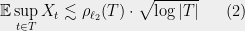
1.2. Method 2:  -nets
-nets
Let  be an -net of under . That is, for all
  there exists
  such that
  . Now note
  so that

Therefore 
We already know  by (2). Also,
  , and
, and

Therefore 
where  denotes the entropy number or covering number, defined as the minimum number of radius-
 balls under metric
  centered at points in required to cover (i.e. the size of the smallest -net). Of course can be chosen to minimize (3). Note the case
  just reduces back to method 1.
1.3. Method 3: Dudley’s inequality (chaining)
The idea of Dudley’s inequality [Dud67] is to, rather than use one net, use a countably infinite sequence of nets. That is, let  denote an
  -net of under , where
 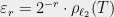 . Let
. Let  denote the closest point in
  to some . Note
  is a valid
  -net. Then

so then 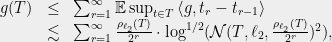
with the last inequality using (2), since the triangle inequality yields 
Thus 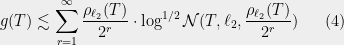
The sum (4) is perfectly fine as is, though the typical formulation of Dudley’s inequality then bounds the sum by an integral over (representing  ) then performs the change of variable
  . This yields the usual formulation of Dudley’s inequality:

It is worth pointing out that Dudley’s inequality is equivalent to the following bound. We say  is an admissible sequence if
  and
and  . Then Dudley’s inequality is equivalent to the bound

To see this most easily, compare with the bound (4). Note that to minimize  , we should pick the best quality net we can using
  points. From
  until some
  , the quality of the net will be, up to a factor of
  , equal to
  , and for the
  in this range the summands of (6) will be a geometric series that sum to
  . Then from
  to some
  , the quality of the best net will be, up to a factor of , equal to
  , and these summands then are a geometric series that sum to
 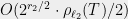 , etc. In this way, the bounds of (4) and (6) are equivalent up to a constant factor.
Note, this is the primary reason we chose the  to have doubly exponential size in : so that the sum of
  in any contiguous range of is a geometric series dominated by the last term.
1.4. Method 4: generic chaining
Here we will show the generic chaining method, which yields the bound of [Fer75], though we will present an equivalent bound that was later given by Talagrand (see his book [Tal14]):
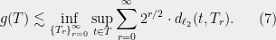
where the infimum is taken over admissible sequences.
Note the similarity between (6) and (7): the latter bound moved the supremum outside the sum. Thus clearly the bound (7) can only be a tighter bound. For a metric , Talagrand defined
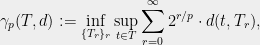
so now we wish to prove the statement 
(You are probably guessing at this point that had we not been working with subgaussians, but rather random variables that have decay bounded by  , we would get a bound in terms of the
  -functional — your guess is right. I leave it to you as an exercise to modify arguments appropriately!)
Now, we have

Note for fixed  , by gaussian decay

for some constant  , since
 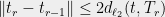 by the triangle inequality.
Therefore
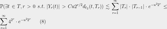
since  . The above sum is convergent for
  .
.
Now, again using that  , we have
![\displaystyle \begin{array}{rcl} g(T) &\le& \int_0^\infty \mathbb{P}(\sup_{t\in T} \sum_{r=1}^\infty Y_r > w) dw\\ {}&\lesssim& \gamma_2(T, \ell_2)\cdot \int_0^\infty \mathbb{P}(\sup_{t\in T}\sum_{r=1}^\infty Y_r > u\cdot C \sup_{t\in T}\sum_{r=1}^\infty 2^{r/2}d_{\ell_2}(t, T_r)) du\text{ (change of variables)}\\ {}&\lesssim& \gamma_2(T, \ell_2)\cdot [2 + \int_2^\infty \mathbb{P}(\sup_{t\in T}\sum_{r=1}^\infty Y_r > u\cdot C \sup_{t\in T}\sum_{r=1}^\infty 2^{r/2}d_{\ell_2}(t, T_r)) du]\\ {}&\le& \gamma_2(T, \ell_2)\cdot [2 + \int_2^\infty \mathbb{P}(\exists t\in T, r>0\ s.t.\ |Y_r(t)| > C u2^{r/2} d_{\ell_2}(t, T_r)) du]\\ {}&\lesssim& \gamma_2(T, \ell_2) \end{array}](https://s0.wp.com/latex.php?latex=%5Cdisplaystyle++%5Cbegin%7Barray%7D%7Brcl%7D++g%28T%29+%26%5Cle%26+%5Cint_0%5E%5Cinfty+%5Cmathbb%7BP%7D%28%5Csup_%7Bt%5Cin+T%7D+%5Csum_%7Br%3D1%7D%5E%5Cinfty+Y_r+%3E+w%29+dw%5C%5C+%7B%7D%26%5Clesssim%26+%5Cgamma_2%28T%2C+%5Cell_2%29%5Ccdot+%5Cint_0%5E%5Cinfty+%5Cmathbb%7BP%7D%28%5Csup_%7Bt%5Cin+T%7D%5Csum_%7Br%3D1%7D%5E%5Cinfty+Y_r+%3E+u%5Ccdot+C+%5Csup_%7Bt%5Cin+T%7D%5Csum_%7Br%3D1%7D%5E%5Cinfty+2%5E%7Br%2F2%7Dd_%7B%5Cell_2%7D%28t%2C+T_r%29%29+du%5Ctext%7B+%28change+of+variables%29%7D%5C%5C+%7B%7D%26%5Clesssim%26+%5Cgamma_2%28T%2C+%5Cell_2%29%5Ccdot+%5B2+%2B+%5Cint_2%5E%5Cinfty+%5Cmathbb%7BP%7D%28%5Csup_%7Bt%5Cin+T%7D%5Csum_%7Br%3D1%7D%5E%5Cinfty+Y_r+%3E+u%5Ccdot+C+%5Csup_%7Bt%5Cin+T%7D%5Csum_%7Br%3D1%7D%5E%5Cinfty+2%5E%7Br%2F2%7Dd_%7B%5Cell_2%7D%28t%2C+T_r%29%29+du%5D%5C%5C+%7B%7D%26%5Cle%26+%5Cgamma_2%28T%2C+%5Cell_2%29%5Ccdot+%5B2+%2B+%5Cint_2%5E%5Cinfty+%5Cmathbb%7BP%7D%28%5Cexists+t%5Cin+T%2C+r%3E0%5C+s.t.%5C+%7CY_r%28t%29%7C+%3E+C+u2%5E%7Br%2F2%7D+d_%7B%5Cell_2%7D%28t%2C+T_r%29%29+du%5D%5C%5C+%7B%7D%26%5Clesssim%26+%5Cgamma_2%28T%2C+%5Cell_2%29+%5Cend%7Barray%7D+&bg=eeeeee&fg=000000&s=0&c=20201002)
as desired.
Surprisingly, Talagrand showed that not only is  an asymptotic upper bound for
  , but it is also an asymptotic lower bound (at least when the entries of are actually gaussians — the lower bound does not hold for subgaussian entries). That is,
  for any . This is known as the “majorizing measures theorem” for reasons we will not get into. In brief: the formulation of [Fer75] did not talk about admissible sequences, or discrete sets at all, but rather worked with measures and provided an upper bound in terms of an infimum over a set of probability measures of a certain integral — this formulation is equivalent to the formulation discussed above in terms of admissible sets, and a proof of the equivalence appears in [Tal14].
1.5. A concrete example
Consider the example  , i.e. the unit
  ball in
  . I picked this example because it is easy to already know using other methods. Why? Well,
  , since the dual norm of
  is ! Thus
  , which one can check is
  . Thus we know the answer is .
So now the question: what do the four methods above give?
Method 1 (union bound): This method gives nothing, since is an infinite set.
Method 2 (-net): To apply this method, we need to understand the size of an -net of the unit ball under . One bound comes from Maurey’s empirical method, which we will not cover here. It implies 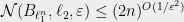 . Another bound is via a volume argument, which we also will not cover here; it implies
  . In short,

By picking  , (3) gives us
  . This is exponentially worse than true bound of
  .
.
Method 3 (Dudley’s inequality):
Combining (9) with (5),

This is exponentially better than method 2, but still off from the truth. We can though wonder: perhaps the issue is not Dudley’s inequality, but perhaps the entropy bounds of (9) are simply loose? Unfortunately this is not the case. To see this, take a set  of vectors in that are each
  -sparse, with
  in each non-zero coordinate, and so that all pairwise distances are
  . A random collection satisfies this distance property with high probability for
  and
and  . Then note
  and furthermore one needs at least
  radius- balls in just to cover . (Thanks to Oded Regev for this simple demonstration.)
It is also worth pointing out that this is the worst case for Dudley’s inequality: it can never be off by more than a factor of  . I’ll leave it to you as an exercise to figure out why (you should assume the majorizing measures theorem, i.e. that (7) is tight)! Hint: compare (6) with (7) and show that nothing interesting happens beyond
  .
.
Method 4 (generic chaining):
By the majorizing measures theorem, we know there must exist an admissible sequence giving the correct  , thus being superior to Dudley’s inequality. I will leave constructing it to you as homework! Note: I know for certain that this is a humanly doable task. Eric Price, Mary Wootters, and I tried at some point in the past as exercise. Eric and I managed to get it down to
  , and Mary then figured out an admissible sequence achieving the optimal
  . So, it’s doable!
Bibliography
[Dud67] Richard M. Dudley. The sizes of compact subsets of Hilbert space and continuity of Gaussian processes. J. Functional Analysis, 1:290–330, 1967.
[Fer75] Xavier Fernique. Regularité des trajectoires des fonctions aléatoires gaussiennes. Lecture Notes in Math., 480:1–96, 1975.
[Tal14] Michel Talagrand. Upper and lower bounds for stochastic processes: modern methods and classical problems. Springer, 2014.

Hi,
In the derivation for the union bound (1.1), I don’t understand where, in the third inequality, the $\rho_{l_2}(T)$ term in the integrand comes from. Could someone please clarify this?
$X_t = \langle t,g \rangle$. Thus $X_t$ is a gaussian with variance $\|t\|_2^2 \le \rho_{l_2}(T)^2$. A gaussian with variance $\sigma^2$ decays like $\exp(-x / (2\sigma^2))$. Does that clarify things?
Sorry, I think the question was why it also shows up as a product instead of just in the denominator of the exponent.
I hope I’m addressing the right concern here (typing from a phone with really bad internet and the original post isn’t loading, so I’m guessing what I wrote before :)).
I think the question is about the following (?). Suppose there are N (possibly dependent) gaussians each with standard deviation at most s. Then the expected max of them is O(s sqrt(lg N)). Are you wondering why? (Here s is rho_{l_2}(T).) The reason is E max(g_1,…,g_N) u) du.
Now you break the integral into two regions: below u* and above u*. For below u*, you just say the integrand is never bigger than 1 (it’s a probability), so you get a contribution of at most u* from small u. For large u, you use a union bound and say Pr(max(..) > u) =u*, you get something like N exp(- C u*^2 / s^2). Now set u* = C’ s sqrt(lg N) to balance the two integrals, and your overall bound becomes O(s sqrt(lg N)).
If I’m understanding your comment right, instead of bounding by N exp(- C u*^2 / s^2), in your post, you’ve bounded it by s * N exp(- C u*^2 / s^2) (note extra factor of s, which is what I was asking about)
You’re right, that’s a typo. That extra factor of $s$ shouldn’t be there. The next line is correct though and seems to have correctly pretended the extra $s$ wasn’t there.
Typo fix: for method 4, in (8) and in a few places before it, the $\exp(-u^2 2^{2^r})$ should be $\exp(-u^2 2^r)$ (thanks to David Woodruff for catching that).
In the example “1.1. Method 1: union bound”, don’t you think that the correct threshold in the integral is $\rho(T) \sqrt{2 \log |T|}$ instead of $C \rho(T) \sqrt{ \log n}$?
With the original threshold, I’m unable to remove the dependence in $|T|$ appearing from the union bound in in the last integral.
Yes, you’re absolutely right. It seems I wrote those lines while thinking that n denoted |T|, whereas I earlier defined n as the dimension. The integral should really go up to some $C \rho(T) \sqrt{\log |T|}$.
Perfect! Thanks for your super fast answer!