Restricted Invertiblity by Interlacing Polynomials

In this post, I am going to give you a simple, self-contained, and fruitful demonstration of a recently introduced proof technique called the method of interlacing families of polynomials, which was also mentioned in an earlier post. This method, which may be seen as an incarnation of the probabilistic method, is relevant in situations when you want to show that at least one matrix from some collection of matrices must have eigenvalues in a certain range. The basic methodology is to write down the characteristic polynomial of each matrix you care about, compute the average of all these polynomials (literally by averaging the coefficients), and then reason about the eigenvalues of the individual matrices by studying the zeros of the average polynomial. The relationship between the average polynomial and the individuals hinges on a phenomenon known as interlacing.

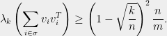
We will use the method to prove the following sharp variant of Bourgain and Tzafriri’s restricted invertibility theorem, which may be seen as a robust, quantitative version of the fact that every rank ${k}$ matrix contains a set of ${k}$ linearly independent columns.

Theorem 1 Suppose ${v_1,\ldots,v_m\in{\mathbb R}^n}$ are vectors with ${\sum_{i=1}^mv_iv_i^T=I_n}$ . Then for every ${k<n}$ there is a subset ${\sigma\subset [m]}$ of size ${k}$ with

$\displaystyle \lambda_k\left(\sum_{i\in\sigma}v_iv_i^T\right)\geq \left(1-\sqrt{\frac{k}{n}}\right)^2\frac{n}{m}.$

That is, any set of vectors ${v_1,\ldots,v_m}$ with variance ${\sum_{i=1}^m \langle x,v_i\rangle^2}$ equal to one in every direction ${\|x\|=1}$ must contain a large subset which is far from being linearly degenerate, in the sense of having large eigenvalues (compared to $(n/m)$ , which is the average squared length of the vectors). Such variance one sets go by many other names in different contexts: they are also called isotropic sets, decompositions of the identity, and tight frames. This type of theorem was first proved by Bourgain and Tzafriri in 1987, and later generalized and sharpened to include the form stated here.

The original applications of Theorem 1 and its variants were mainly in Banach space theory and harmonic analysis. More recently, it was used in theoretical CS by Nikolov, Talwar, and Zhang in the contexts of differential privacy and discrepancy minimization. Another connection with TCS was discovered by Joel Tropp, who showed that the set ${\sigma}$ can be found algorithmically using a semidefinite program whose dual is related to the Goemans-Wiliamson SDP for Max-Cut.

In more concrete notation, the theorem says that every rectangular matrix ${B_{n\times m}}$ with ${BB^T=I_n}$ contains an ${n\times k}$ column submatrix ${S\subset [m]}$ with ${\sigma_k^2(B_S)\ge (1-\sqrt{k/n})^2(n/m)}$ , where ${\sigma_k}$ is the kth largest singular value. Written this way, we see some similarity with the column subset selection problem in data mining, which seeks to extract a maximally nondegenerate set of `representative’ columns from a data matrix. There are also useful generalizations of Theorem 1 for arbitrary rectangular ${B}$ .

As I said earlier, the technique is based on studying the roots of averages of polynomials. In general, averaging polynomials coefficient-wise can do unpredictable things to the roots. For instance, the average of ${(x-1)(x-2)}$ and ${(x-3)(x-4)}$ , which are both real-rooted quadratics, is ${x^2-5x+7}$ , which has complex roots ${2.5\pm\sqrt{3}i}$ . Even when the roots of the average are real, there is in general no simple relationship between the roots of two polynomials and the roots of their average.

The main insight is that there are nonetheless many situations where averaging the coefficients of polynomials also has the effect of averaging each of the roots individually, and that it is possible to identify and exploit these situations. To speak about this concretely, we will need to give the roots names. There is no canonical way to do this for arbitrary polynomials, whose roots are just sets of points in the complex plane. However, when all the roots are real there is a natural ordering given by the real line; we will use this ordering to label the roots of a real-rooted polynomial 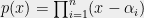${p(x)=\prod_{i=1}^n (x-\alpha_i)}$ in descending order ${\alpha_1\ge\ldots\ge\alpha_n}$ .

Interlacing

We will use the following classical notion to characterize precisely the good situations mentioned above.

Definition 2 (Interlacing) Let ${f}$ be a degree ${n}$ polynomial with all real roots ${\{\alpha_i\}}$ , and let ${g}$ be degree ${n}$ or ${n-1}$ with all real roots ${\{\beta_i\}}$ (ignoring ${\beta_n}$ in the degree ${n-1}$ case). We say that ${g}$ interlaces ${f}$ if their roots alternate, i.e.,

$\displaystyle \beta_n\le\alpha_n\le \beta_{n-1}\le \ldots \beta_1\le \alpha_1.$

Following Fisk, we denote this as ${g\longrightarrow f}$ , to indicate that the largest root belongs to ${f}$ .

If there is a single ${g}$ which interlaces a family of polynomials ${f_1,\ldots,f_m}$ , we say that they have a common interlacing.

It is an easy exercise that 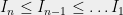${f_1,\ldots,f_m}$ of degree ${n}$ have a common interlacing iff there are closed intervals ${I_n\le I_{n-1}\le\ldots I_1}$ (where ${\le}$ means to the left of) such that the ${i}$ th roots of all the ${f_j}$ are contained in ${I_i}$ . It is also easy to see that a set of polynomials has a common interlacing iff every pair of them has a common interlacing (this may be viewed as Helly’s theorem on the real line).

We now state the main theorem about averaging polynomials with common interlacings.

Theorem 3 Suppose ${f_1,\ldots,f_m}$ are real-rooted of degree ${n}$ with positive leading coefficients. Let ${\lambda_k(f_j)}$ denote the ${k^{th}}$ largest root of ${f_j}$ and let ${\mu}$ be any distribution on ${[m]}$ . If ${f_1,\ldots,f_m}$ have a common interlacing, then for all ${k=1,\ldots,n}$

$\displaystyle \min_j \lambda_k(f_j)\le \lambda_k(\mathop{\mathbb E}_{j\sim \mu} f_j)\le \max_j \lambda_k(f_j).$

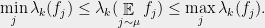
The proof of this theorem is a three line exercise. Since it is the crucial fact upon which the entire technique relies, I encourage you to find this proof for yourself (Hint: Apply the intermediate value theorem inside each interval ${I_i}$ .) You can also look at the picture below, which shows what happens for two cubic polynomials with a quadratic common interlacing.

One of the nicest features of common interlacings is that their existence is equivalent to certain real-rootedness statements. Often, this characterization gives us a systematic way to argue that common interlacings exist, rather than having to rely on cleverness and pull them out of thin air. The following seems to have been discovered a number of times (for instance, Fell or Chudnovsky & Seymour); the proof of it included below assumes that the roots of a polynomial are continuous functions of its coefficients (which may be shown using elementary complex analysis).

Theorem 4 If ${f_1,\ldots,f_m}$ are degree ${n}$ polynomials and all of their convex combinations ${\sum_{i=1}^m \mu_if_i}$ have real roots, then they have a common interlacing.

Proof: Since common interlacing is a pairwise condition, it suffices to handle the case of two polynomials ${f_0}$ and ${f_1}$ . Let

$\displaystyle f_t := (1-t)f_0+tf_1$

with ${t\in [0,1]}$ . Assume without loss of generality that ${f_0}$ and ${f_1}$ have no common roots (if they do, divide them out and put them back in at the end). As ${t}$ varies from ${0}$ to ${1}$ , the roots of ${f_t}$ define ${n}$ continuous curves in the complex plane ${C_1,\ldots,C_n}$ , each beginning at a root of ${f_0}$ and ending at a root of ${f_1}$ . By our assumption the curves must all lie in the real line. Observe that no curve can cross a root of either ${f_0}$ or ${f_1}$ in the middle: if ${f_t(r)=0}$ for some ${t \in (0,1)}$ and ${f_0(r)=0}$ , then immediately we also have ${f_t(r)=tf_1(r)=0}$ , contradicting the no common roots assumption. Thus, each curve defines a closed interval containing exactly one root of ${f_0}$ and one root of ${f_1}$ , and these intervals do not overlap except possibly at their endpoints, establishing the existence of a common interlacing. $\Box$

Characteristic Polynomials and Rank One Updates

A very natural and relevant example of interlacing polynomials comes from matrices. Recall that the characteristic polynomial of a matrix ${A}$ is given by

$\displaystyle \chi(A)(x):=\det(xI-A)$

and that its roots are the eigenvalues of ${A}$ . The following classical fact tells us that rank one updates create interlacing.

Lemma 5 (Cauchy’s Interlacing Theorem) If ${A}$ is a symmetric matrix and ${v}$ is a vector then

$\displaystyle \chi(A)\longrightarrow \chi(A+vv^T).$

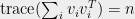
Proof: There are many ways to prove this, and it is a nice exercise. One way which I particularly like, and which will be relevant for the rest of this post, is to observe that

$\displaystyle \begin{array}{rcl} \det(xI-A-vv^T) &= \det(xI-A)\det(I-vv^T(xI-A)^{-1})\qquad (*) \\&=\det(xI-A)(1-v^T(xI-A)^{-1}v) \\&=\chi(A)(x)\left(1-\sum_{i=1}^n\frac{\langle v,u_i\rangle^2}{x-\lambda_i}\right),\end{array}$

where ${u_i}$ and ${\lambda_i}$ are the eigenvectors and eigenvalues of ${A}$ . Interlacing then follows by inspecting the poles and zeros of the rational function on the right hand side. $\Box$

We are now in a position to do something nontrivial. Suppose ${A}$ is a symmetric ${n\times n}$ real matrix and ${v_1,\ldots,v_m}$ are some vectors in ${{\mathbb R}^n}$ . Cauchy’s theorem tells us that the polynomials

$\displaystyle \chi(A+v_1v_1^T),\chi(A+v_2v_2^T),\ldots,\chi(A+v_mv_m^T)$

have a common interlacing, namely ${\chi(A)}$ . Thus, Theorem 3 implies that for every ${k}$ , there exists a ${j}$ so that the ${k}$ th largest eigenvalue of ${A+v_jv_j^T}$ is at least the ${k}$ th largest root of the average polynomial

$\displaystyle \mathop{\mathbb E}_j \chi(A+v_jv_j^T).$

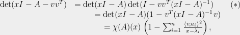
We can compute this polynomial using the calculation ${(*)}$ as follows:

$\displaystyle \mathop{\mathbb E} \chi(A+v_jv_j^T) = \chi(A)\left(1-\sum_{i=1}^n\frac{ \mathop{\mathbb E} \langle v_j,u_i\rangle^2}{x-\lambda_i}\right).$

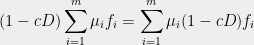
In general, this polynomial depends on the squared inner products ${\langle v_j,u_i\rangle^2}$ . When ${\sum_{i=1}^m v_iv_i^T=I}$ , however, we have ${\mathop{\mathbb E}_j \langle v_j,u_i\rangle^2=1/m}$ for all ${u_i}$ , and:

$\displaystyle \mathop{\mathbb E}_j \chi(A+v_jv_j^T) = \chi(A)(x)\left(1-\sum_{i=1}^n\frac{ 1/m}{x-\lambda_i}\right)=\chi(A)(x)-(1/m)\frac{\partial}{\partial x}\chi(A)(x).\qquad (**)$

That is, adding a random rank one matrix in the isotropic case corresponds to subtracting off a multiple of the derivative from the characteristic polynomial. Note that there is no dependence on the vectors ${v_j}$ in this expression, and it has `forgotten’ all of the eigenvectors ${u_i}$ . This is where the gain is: we have reduced a high-dimensional linear algebra problem (of finding a ${v_j}$ for which ${A+v_jv_j^T}$ has certain eigenvalues, which may be difficult when the matrices involved do not commute) to a univariate calculus / analysis problem (given a polynomial, figure out what subtracting the derivative does to its roots). Moreover, the latter problem is amenable to a completely different set of tools than the original eigenvalue problem.

As a sanity check, if we apply the above deduction to ${A=0}$ , we find that any isotropic set ${\sum_{i=1}^m v_iv_i^T=I}$ must contain a ${j}$ such that ${\lambda_1(v_jv_j^T)}$ is at least the largest root of

$\displaystyle \chi(0)(x)-(1/m)\chi(0)'(x)=x^n-(n/m)x^{n-1},$

which is just ${n/m}$ . This makes sense since ${\lambda_1(v_jv_j^T)=\|v_j\|^2}$ , and the average squared length of the vectors is indeed ${n/m}$ since ${\mathrm{trace}(\sum_i v_iv_i^T)=n}$ .

Differential Operators and Induction

The real power of the method comes from being able to apply it inductively to a sum of many independent random ${v_j}$ ‘s at once, rather than just once. In this case, establishing the necessary common interlacings requires a combination of Theorem 4 and Cauchy’s theorem. A central role is played by the differential operators ${(I-(1/m)\frac{\partial}{\partial x})}$ seen above, which I will henceforth denote as ${(I-(1/m)D)}$ . The proof relies on the following key properties of these operators:

Lemma 6 (Properties of Differential Operators)

If ${ \mathbf{X} }$ is a random vector with ${\mathop{\mathbb E} \mathbf{X} \mathbf{X} ^T = cI}$ then
$\displaystyle \mathop{\mathbb E} \chi(A+ \mathbf{X} \mathbf{X} ^T) = (I-cD)\chi(A).$

If ${f}$ has real roots then so does ${(I-cD)f}$ .

If ${f_1,\ldots,f_m}$ have a common interlacing, then so do ${(I-cD)f_1,\ldots, (1-cD)f_m}$ .

Proof: Part (1) was essentially shown in ${(**)}$ . Part (2) follows by applying ${(*)}$ to the matrix ${A}$ with diagonal entries equal to the roots of ${f}$ , and plugging in ${v=\sqrt{c}\cdot(1,1,\ldots,1)^T}$ , so that ${f=\chi[A]}$ and ${(1-cD)f=\chi[A+vv^T]}$ .

For part (3), Theorem 3 tells us that all convex combinations ${\sum_{i=1}^m\mu_if_i}$ have real roots. By part (2) it follows that all

$\displaystyle (1-cD)\sum_{i=1}^m\mu_if_i = \sum_{i=1}^m \mu_i (1-cD)f_i$

also have real roots. By Theorem 4, this means that the ${(1-cD)f_i}$ must have a common interlacing. $\Box$

We are now ready to perform the main induction which will give us the proof of Theorem 1.

Lemma 7 Let ${ \mathbf{X} }$ be uniformly chosen from ${\{v_i\}_{i\le m}}$ so that ${\mathop{\mathbb E} \mathbf{X} \mathbf{X} ^T=(1/m)I}$ , and let ${ \mathbf{X} _1,\ldots, \mathbf{X} _k}$ be i.i.d. copies of ${ \mathbf{X} }$ . Then there exists a choice of indices ${j_1,\ldots j_k}$ satisfying

$\displaystyle \lambda_k \left(\chi(\sum_{i=1}^k v_{j_i}v_{j_i}^T)\right) \ge \lambda_k \left(\mathop{\mathbb E} \chi(\sum_{i=1}^k \mathbf{X} _i \mathbf{X} _i^T)\right).$

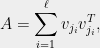
Proof: For any partial assignment ${j_1,\ldots,j_\ell}$ of the indices, consider the `conditional expectation’ polynomial:

$\displaystyle q_{j_1,\ldots,j_\ell}(x) := \mathop{\mathbb E}_{ \mathbf{X} _{\ell+1},\ldots, \mathbf{X} _k} \chi\left(\sum_{i=1}^\ell v_{j_i}v_{j_i}^T + \sum_{i=\ell+1}^k \mathbf{X} _i \mathbf{X} _i^T\right).$

We will show that there exists a ${j_{\ell+1}\in [m]}$ such that

$\displaystyle \lambda_k(q_{j_1,\ldots,j_{\ell+1}})\ge \lambda_k(q_{j_1,\ldots,j_\ell}),\ \ \ \ \ (1)$

which by induction will complete the proof. Consider the matrix

$\displaystyle A = \sum_{i=1}^\ell v_{j_i}v_{j_i}^T,$

By Cauchy’s interlacing theorem 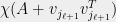${\chi(A)}$ interlaces ${\chi(A+v_{j_{\ell+1}}v_{j_{\ell+1}}^T)}$ for every ${j_{\ell+1}\in [m]}$ . Lemma 6 tells us ${(1-(1/m)D)}$ operators preserve common interlacing, so the polynomials

$\displaystyle (1-(1/m)D)^{k-(\ell+1)}\chi(A+v_{j_{\ell+1}}v_{j_{\ell+1}}^T) = q_{j_1,\ldots,j_\ell,j_{\ell+1}}(x)$

(by applying Lemma 6 ${k-(\ell+1)}$ times) must also have a common interlacing. Thus, some ${j_{\ell+1}\in [m]}$ must satisfy (1), as desired. $\Box$

Bounding the Roots: Laguerre Polynomials

To finish the proof of Theorem 1, it suffices by Lemma 7 to prove a lower bound on the ${k}$ th largest root of the expected polynomial ${\mathop{\mathbb E} \chi\left(\sum_{i=1}^k \mathbf{X} _i \mathbf{X} _i^T\right)}$ . By applying Lemma 6 ${k}$ times to ${\chi(0)=x^n}$ , we find that

$\displaystyle \mathop{\mathbb E} \chi\left(m\cdot \sum_{i=1}^k \mathbf{X} _i \mathbf{X} _i^T\right) = (1-D)^kx^n =: p_k(x).\ \ \ \ \ (2)$

This looks like a nice polynomial, and we are free to use any method we like to bound its roots.

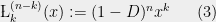
The easiest way is to observe that

$\displaystyle p_k(x)=x^{n-k}\L_k^{(n-k)}(x),$

where ${\L_k^{(n-k)}(x)}$ is a degree ${k}$ associated Laguerre polynomial. These are a classical family of orthogonal polynomials and a lot is known about the locations of their roots; in particular, there is the following estimate due to Krasikov.

Lemma 8 (Roots of Laguerre Polynomials) The roots of the associated Laguerre polynomial

$\displaystyle \L_k^{(n-k)}(x):= (1-D)^{n}x^k\ \ \ \ \ (3)$

are contained in the interval ${[n(1-\sqrt{k/n})^2,n(1+\sqrt{k/n})^2].}$

It follows by Lemma 8 that ${\lambda_k(p_k)\ge \lambda_k(\L_k^{(n-k)})\ge n(1-\sqrt{k/n})^2}$ , which immediately yields Theorem 1 by Lemma 7 and (2).

If you think that appealing to Laguerre polynomials was magical, it is also possible to prove the bound (3) from scratch in less than a page using the `barrier function’ argument from this paper, which is also intimately related to the formulas ${(*)}$ and ${(**)}$ .

Conclusion

The argument given here is a special case of a more general principle: that expected characteristic polynomials of certain random matrices can be expressed in terms of differential operators, which can then be used to establish the existence of the necessary common interlacings as well as to analyze the roots of the expected polynomials themselves. In the isotropic case of Bourgain-Tzafriri presented here, all of these objects can be chosen to be univariate polynomials. Morally, this is because the covariance matrices of all of the random vectors involved are multiples of the identity (which trivially commute with each other), and all of the characteristic polynomials involved are simple univariate linear transformations of each other (such a ${(I-cD)}$ ). The above argument can also be made to work in the non-isotropic case, yielding improvements over previously known bounds. This is the subject of a paper in preparation, Interlacing Families III, with Adam Marcus and Dan Spielman.

On the other hand, the proofs of Kadison-Singer and existence of Ramanujan graphs involve analyzing sums of independent rank one matrices which come from non-identically distributed distributions whose covariance matrices do not commute. At a high level, this is what creates the need to consider multivariate characteristic polynomials and differential operators, which are then analyzed using techniques from the theory of real stable polynomials.

Acknowledgments

Everything in this post is joint work with Adam Marcus and Dan Spielman. Thanks to Raghu Meka for helpful comments in the preparation of this post.

UPDATE: In response to Olaf’s comment below, here is how to see that the bound in the theorem is sharp.

The tight example is provided by random matrices. Let ${G}$ be an ${n\times m}$ random matrix with i.i.d. ${N(0,1/m)}$ Gaussian random entries, so that ${\mathbb{E} A=\mathbb{E} GG^T = I_n}$ . Then ${A}$ is called a Wishart matrix and its spectrum is very well-understood. In particular, we will use the following two facts:

(1) If $m,n\rightarrow\infty$ with ${m/n\rightarrow\infty}$ then the ratio

$\displaystyle \lambda_{1}(A)/\lambda_n(A)\rightarrow 1$

almost surely. Thus, if we take the ${v_i}$ to be the columns of such a ${G}$ then

$\displaystyle \sum_{i=1}^m v_iv_i^T=I(1+o(1))$

almost surely.

(2)If ${m,n\rightarrow\infty}$ with ${n/m=a}$ fixed, the spectrum of ${A}$ converges to a known distribution called the Marchenko-Pastur law, which is supported on the interval ${[(1-\sqrt{a})^2,(1+\sqrt{a})^2]}$ . The eigenvalues are extremely (better than exponentially) unlikely to be supported on any interval smaller than this; in particular for every ${\epsilon>0}$ we have

$\displaystyle \mathbb{P} [\lambda_{n}(A)>(1-\sqrt{a})^2+\epsilon]<\exp(-c(\epsilon)n^2)$

for sufficiently large ${n}$ . This is established in Hiai-Petz (Theorem 8, thanks to S. Szarek for this crucial reference.)

Fact (2) implies that every ${n\times k}$ submatrix ${S}$ of ${G}$ , $k < n$ , which is also Gaussian, has

$\displaystyle \lambda_k(SS^T)<\left((1-\sqrt{a})^2+\epsilon\right)\frac{n}{m}\quad (+)$

with probability $1-{\exp(-ck^2)}$ for sufficiently large ${n}$ (keeping ${k/n}$ fixed). There are ${\binom{m}{k}=\exp(c'k\log(m/k))}$ such submatrices ${S}$ , so if we set $m=n^{3/2}$ (say) then $k^2 >> k\log(m/k)$ for any $k=\Omega(n)$ , and by a union bound $(+)$ holds simultaneously for all $n \times k$ submatrices of G, showing that the guarantee of the theorem cannot be improved for sufficiently large $n$ .

It would be nice to have an argument for finite $n$ , which would require a non-asymptotic version of the Hiai-Petz bound.

10 thoughts on “Restricted Invertiblity by Interlacing Polynomials”

Pingback: Discrepancy, Graphs, and the Kadison-Singer Problem | Windows On Theory
Olaf Mordhorst says:

April 28, 2014 at 8:22 am

Dear Mr Srivastava,

You’ve claimed that your version of the restricted invertibility THM is sharp. Could You tell me for which k this result is sharp and how to see this.

Best regards,
Olaf Mordhorst

1. Nikhil Srivastava says:
  
  April 29, 2014 at 7:06 pm
  
  Dear Olaf,
  That is an excellent question! I have added a section to the post, describing the sense in which the bound is sharp.
  Best wishes,
  Nikhil
  
Pierre Youssef says:

April 29, 2014 at 6:45 pm

Dear Nikhil,

Thank you for this post. It was never clear to me whether the dependence is optimal in the restricted invertibility principle. The argument you present here is very clear. By the way: A=GG^T without expectation. After equation (+), I think it should be with probability bigger than 1-\exp(-ck^2). Also the line just after should be \exp(c’k\log(m/k)).

Also did you try to get simultaneously a lower and upper bound for the singular values of the restricted matrix i.e. to get a well conditionned submatrix in the same sense of what is done here: http://arxiv.org/pdf/1212.0976v2.pdf

Best wishes,
Pierre

1. Nikhil Srivastava says:
  
  April 29, 2014 at 6:57 pm
  
  Thanks, Pierre! Fixed.
  
  Your paper looks very interesting. I have not tried to get both bounds at once using this method for this regime of k, although in some sense that is what is done for k>n in the case of Kadison-Singer. The basic idea is to embed an upper and lower bound into a single matrix by using a direct sum. It would be interesting to see if your result can be obtained using polynomials.
  
Olaf Mordhorst says:

May 7, 2014 at 11:30 am

Dear Nikhil,
Thank you very much for your comment. I’d failed to construct a counter example (by considering Hadamard basis), so your post helped me a lot. Maybe, one can construct a finite counter example by quantizing the gauss measure in your example (since the counter example does only depend on the distribution of the column vectors in G, which might be predictable for m>>n).
Bets wishes,
Olaf

Brad says:

June 3, 2014 at 3:56 pm

This is a very nice blog post! It really helped me understand what’s going on with the method. I don’t think anyone will be confused by it for very long, but I think there is a small typo in equation (3), by the way.

Sanjeev Arora says:

June 10, 2014 at 2:53 pm

Beautiful exposition, Nikhil! I’ve seen this explained a few times and this writeup nails it.

Dorin Dutkay says:

October 25, 2016 at 8:58 am

Dear Nikhil,
Thank you for the very nice exposition, it made the proof of Kadison-Singer much more intuitive for me. I have a question, if you have time to answer it: when you prove Theorem 1 from Lemma 7, the indices j_1,…, j_k might not be mutually distinct. Right? So in Theorem 1, we allow a vector v_i to appear several times in the last inequality?
Many thanks and best wishes,
Dorin

Dorin Dutkay says:

October 31, 2016 at 8:57 am

Hi Nikhil,
Nevermind the previous question, I read the notation wrongly. All clear now. Thanks again for the nice post!
Dorin

	James Cross on GPT as an “Intelligence…
	Thoughts on AI safet… on AI will change the world, but…
	Anonymous on An alarming trend in K-12 Math…
	Interview about this… on Men in Computer Science
	Interview about this… on The Swiss Army Knife of C…

Restricted Invertiblity by Interlacing Polynomials

Published by Nikhil Srivastava

10 thoughts on “Restricted Invertiblity by Interlacing Polynomials”

Leave a Reply to Nikhil Srivastava Cancel reply

Share this:

Like this:

Related

Published by Nikhil Srivastava

10 thoughts on “Restricted Invertiblity by Interlacing Polynomials”

Leave a Reply to Nikhil Srivastava Cancel reply