(This post from the lecture by Yueqi Sheng)
In this post, we will talk about detecting phase transitions using
Approximate-Message-Passing (AMP), which is an extension of
Belief-Propagation to “dense” models. We will also discuss the Replica
Symmetric trick, which is a heuristic method of analyzing phase
transitions. We focus on the Rademacher spiked Wigner model (defined
below), and show how both these methods yield the same phrase transition
in this setting.
The Rademacher spiked Wigner model (RSW) is the following. We are given
observations 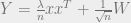


Gaussian-Orthogonal-Ensemble (GOE) matrix:


ratio. The goal is to approximately recover 
The question here is: how small can
impossible to recover anything reasonably correlated with the
ground-truth
(or the replica method) have to say about this?
To answer the first question, one can think of the task here is to
distinguish 

look at the spectrum of the observation matrix 
out that this is an asymptotically optimal distinguisher [1]). The spectrum of
- When
, the empirical distribution of eigenvalues in
spiked model still follows the semicircle law, with the top
eigenvalues -
When
, we start to see an eigenvalue
in the
planted model.

Approximate message passing
This section approximately follows the exposition in [3].
First, note that in the Rademacher spiked Wigner model, the posterior
distribution of the signal 
is: ![\Pr[\sigma | Y] \propto \Pr[Y | \sigma] \propto \prod_{i \neq j} \exp(\lambda Y_{i, j} \sigma_i \sigma_j /2 )](https://s0.wp.com/latex.php?latex=%5CPr%5B%5Csigma+%7C+Y%5D+%5Cpropto+%5CPr%5BY+%7C+%5Csigma%5D+%5Cpropto+%5Cprod_%7Bi+%5Cneq+j%7D+%5Cexp%28%5Clambda+Y_%7Bi%2C+j%7D+%5Csigma_i+%5Csigma_j+%2F2+%29&bg=eeeeee&fg=666666&s=0&c=20201002)
defines a graphical-model (or “factor-graph”), over which we can perform
Belief-Propogation to infer the posterior distribution of
However, in this case the factor-graph is dense (the distribution is a
product of potentials 
pairs of 
In the previous blog post, we saw belief propagation works great when the underlying interaction
graph is sparse. Intuitively, this is because 
which allows us to assume each messages are independent random
variables. In dense model, this no longer holds. One can think of dense
model as each node receive a weak signal from all its neighbors.
In the dense model setting, a class of algorithms called Approximate
message passing (AMP) is proposed as an alternative of BP. We will
define AMP for RWM in terms of its state evolution.
State evolution of AMP for Rademacher spiked Wigner model
Recall that in BP, we wish to infer the posterior distributon of
probability distribution over values on nodes. In our setting, since the
distributions are over 
their expected values. Let ![m^t_{u \to v} \in [-1, 1]](https://s0.wp.com/latex.php?latex=m%5Et_%7Bu+%5Cto+v%7D+%5Cin+%5B-1%2C+1%5D&bg=eeeeee&fg=666666&s=0&c=20201002)
message from 


to the expected value ![{{\mathbb{E}}}[\sigma_u]](https://s0.wp.com/latex.php?latex=%7B%7B%5Cmathbb%7BE%7D%7D%7D%5B%5Csigma_u%5D&bg=eeeeee&fg=666666&s=0&c=20201002)
To derive the BP update rules, we want to compute the expectation
![{{\mathbb{E}}}[\sigma_v]](https://s0.wp.com/latex.php?latex=%7B%7B%5Cmathbb%7BE%7D%7D%7D%5B%5Csigma_v%5D&bg=eeeeee&fg=666666&s=0&c=20201002)
messages 
do this using the posterior distribution of the RWM, ![\Pr[\sigma | Y]](https://s0.wp.com/latex.php?latex=%5CPr%5B%5Csigma+%7C+Y%5D&bg=eeeeee&fg=666666&s=0&c=20201002)
which we computed above.
![\displaystyle \Pr[\sigma_v = 1 | Y, \{\sigma_u\}_{u \neq v}] = \frac{ \prod_u \exp(\lambda Y_{u, v} \sigma_u) - \prod_u \exp(-\lambda Y_{u, v} \sigma_u) }{ \prod_u \exp(\lambda Y_{u, v} \sigma_u) + \prod_u \exp(-\lambda Y_{u, v} \sigma_u) }](https://s0.wp.com/latex.php?latex=%5Cdisplaystyle+%5CPr%5B%5Csigma_v+%3D+1+%7C+Y%2C+%5C%7B%5Csigma_u%5C%7D_%7Bu+%5Cneq+v%7D%5D+%3D+%5Cfrac%7B+%5Cprod_u+%5Cexp%28%5Clambda+Y_%7Bu%2C+v%7D+%5Csigma_u%29+-+%5Cprod_u+%5Cexp%28-%5Clambda+Y_%7Bu%2C+v%7D+%5Csigma_u%29+%7D%7B+%5Cprod_u+%5Cexp%28%5Clambda+Y_%7Bu%2C+v%7D+%5Csigma_u%29+%2B+%5Cprod_u+%5Cexp%28-%5Clambda+Y_%7Bu%2C+v%7D+%5Csigma_u%29+%7D&bg=eeeeee&fg=666666&s=0&c=20201002)
And similarly for ![\Pr[\sigma_v = -1 | Y, \{\sigma_u\}_{u \neq v}]](https://s0.wp.com/latex.php?latex=%5CPr%5B%5Csigma_v+%3D+-1+%7C+Y%2C+%5C%7B%5Csigma_u%5C%7D_%7Bu+%5Cneq+v%7D%5D&bg=eeeeee&fg=666666&s=0&c=20201002)
From the above, we can take expectations over 
![\{{{\mathbb{E}}}[\sigma_u]\}_{u \neq v}](https://s0.wp.com/latex.php?latex=%5C%7B%7B%7B%5Cmathbb%7BE%7D%7D%7D%5B%5Csigma_u%5D%5C%7D_%7Bu+%5Cneq+v%7D&bg=eeeeee&fg=666666&s=0&c=20201002)
using the heuristic assumption that the distribution of
product distribution), we find that the BP state update can be written
as:
where the interaction matrix 


Now, Taylor expanding 

since the terms 

At this point, we could try dropping the “non-backtracking” condition


depend on receiver – so we write 
However, this simplification turns out not to work for estimating the
signal. The problem is that the “backtracking” terms which we added
amplify over two iterations.
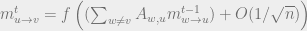
In AMP, we simply perform the above procedure, except we add a
correction term to account for the backtracking issue above. Given
for all
![m^{t}_{u \to v} = m^{t}_u = f(\sum_{w}A_{w, u} m^{t - 1}_{w}) + [\text{some correction term}]](https://s0.wp.com/latex.php?latex=m%5E%7Bt%7D_%7Bu+%5Cto+v%7D+%3D+m%5E%7Bt%7D_u+%3D+f%28%5Csum_%7Bw%7DA_%7Bw%2C+u%7D+m%5E%7Bt+-+1%7D_%7Bw%7D%29+%2B+%5B%5Ctext%7Bsome+correction+term%7D%5D&bg=eeeeee&fg=666666&s=0&c=20201002)
The correction term corresponds to error introduced by the backtracking
terms. Suppose everything is good until step 
the influence of backtracking term to a node
At time 

each of it’s neighbor


this error term is to large to ignore. To characterize the exact form of
correction, we simply do a taylor expansion
State evolution of AMP
In this section we attempt to obtain the phase transition of Rademacher
spiked Wigner model via looking at 
We assume that each message could be written as a sum of signal term and
noise term. 

transition), we need to look at how the signal 

We do the following simplification: ignore the correction term and
assume each time we obtain an independent noise 

Here, we see that
and 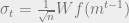

Note that 
ground truth and current belief, since the function 
magnitude of the current beliefs bounded.
![\frac{\lambda}{n} <f(m^{t - 1}), x>= \frac{\lambda}{n} <f(\mu_{t - 1}x + \sigma_{t - 1}g), x> \approx\lambda {{\mathbb{E}}}_{X \sim unif(\pm 1), G\sim \mathbb{N}(0, 1)}[X f(\mu_{t - 1}X + \sigma_{t - 1}G)] = \lambda {{\mathbb{E}}}_G[f(\mu_{t - 1} + \sigma_{t - 1}G)]](https://s0.wp.com/latex.php?latex=%5Cfrac%7B%5Clambda%7D%7Bn%7D+%3Cf%28m%5E%7Bt+-+1%7D%29%2C+x%3E%3D+%5Cfrac%7B%5Clambda%7D%7Bn%7D+%3Cf%28%5Cmu_%7Bt+-+1%7Dx+%2B+%5Csigma_%7Bt+-+1%7Dg%29%2C+x%3E+%5Capprox%5Clambda+%7B%7B%5Cmathbb%7BE%7D%7D%7D_%7BX+%5Csim+unif%28%5Cpm+1%29%2C+G%5Csim+%5Cmathbb%7BN%7D%280%2C+1%29%7D%5BX+f%28%5Cmu_%7Bt+-+1%7DX+%2B+%5Csigma_%7Bt+-+1%7DG%29%5D+%3D+%5Clambda+%7B%7B%5Cmathbb%7BE%7D%7D%7D_G%5Bf%28%5Cmu_%7Bt+-+1%7D+%2B+%5Csigma_%7Bt+-+1%7DG%29%5D&bg=eeeeee&fg=666666&s=0&c=20201002)
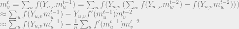
For the noise term, each coordinate of
variable with
![\frac{1}{n} \sum_v f(m^{t - 1})_v^2 \approx {{\mathbb{E}}}_{X, G}[f(\mu_{t - 1}X + \sigma_{t - 1}G)^2] = {{\mathbb{E}}}_{G}[f(\mu_{t - 1} + \sigma_{t - 1}G)^2]](https://s0.wp.com/latex.php?latex=%5Cfrac%7B1%7D%7Bn%7D+%5Csum_v+f%28m%5E%7Bt+-+1%7D%29_v%5E2+%5Capprox+%7B%7B%5Cmathbb%7BE%7D%7D%7D_%7BX%2C+G%7D%5Bf%28%5Cmu_%7Bt+-+1%7DX+%2B+%5Csigma_%7Bt+-+1%7DG%29%5E2%5D+%3D+%7B%7B%5Cmathbb%7BE%7D%7D%7D_%7BG%7D%5Bf%28%5Cmu_%7Bt+-+1%7D+%2B+%5Csigma_%7Bt+-+1%7DG%29%5E2%5D&bg=eeeeee&fg=666666&s=0&c=20201002)
It was shown in [4] that we can introduce a new
parameter 
As 


![\gamma_t = \lambda^2 {{\mathbb{E}}}[f(\gamma_{t - 1} + \sqrt{\gamma_{t - 1}}G)]](https://s0.wp.com/latex.php?latex=%5Cgamma_t+%3D+%5Clambda%5E2+%7B%7B%5Cmathbb%7BE%7D%7D%7D%5Bf%28%5Cgamma_%7Bt+-+1%7D+%2B+%5Csqrt%7B%5Cgamma_%7Bt+-+1%7D%7DG%29%5D&bg=eeeeee&fg=666666&s=0&c=20201002)
This heuristic analysis of AMP actually gives a phase transition at

- For
: If
,
w.h.p., thus we have
. Taking
, which means there AMP solution has no overlap with the ground truth.
-
For
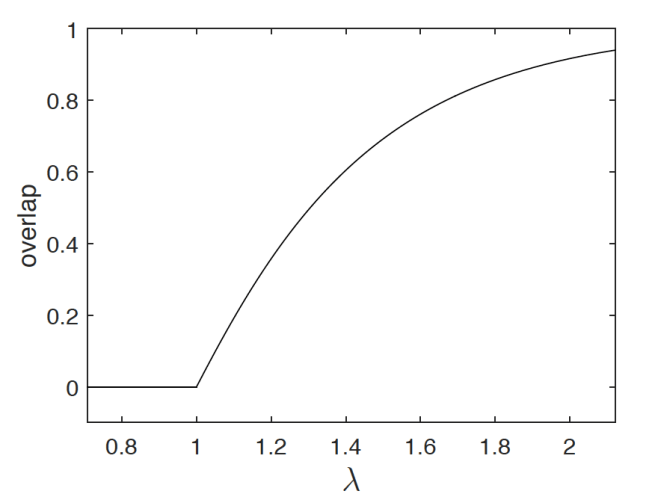
(Figure from [6])
Replica symmetry trick
Another way of obtaining the phase transition is via a non-rigorous
analytic method called the replica method. Although non-rigorous, this
method from statistical physics has been used to predict the fixed point
of many message passing algorithms and has the advantage of being easy
to simulate. In our case, we will see that we obtain the same phase
transition temperature as AMP above. The method is non-rigorous due to
several assumptions made during the computation.
Outline of replica method
Recall that we are interested in minizing the free energy of a given
system 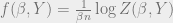

the partition function as before:


In replica method,
assumption is that as 
too much, so we will look at the mean of 
energy of the system.
![f(\beta) = \lim_{n \to \infty}\frac{1}{\beta n}{{\mathbb{E}}}_{Y}[\log Z(\beta, Y)]](https://s0.wp.com/latex.php?latex=f%28%5Cbeta%29+%3D+%5Clim_%7Bn+%5Cto+%5Cinfty%7D%5Cfrac%7B1%7D%7B%5Cbeta+n%7D%7B%7B%5Cmathbb%7BE%7D%7D%7D_%7BY%7D%5B%5Clog+Z%28%5Cbeta%2C+Y%29%5D&bg=eeeeee&fg=666666&s=0&c=20201002)

compute the free energy density as a function of only 
temperature of the system.
The replica method is first proposed as a simplification of the
computation of
It is a generally hard problem to compute
naive attempt of approximate
Unfortunately 
at least when temperature is low. Intuitively,
system with a fixed
fluctuate together. When the temperature is high,
roll in system thus they could be close. However, when temperature is
low, there could be a problems. Let 


![g(\beta) = \frac{1}{\beta n}\log {{\mathbb{E}}}_Y[Z(\beta, Y)]](https://s0.wp.com/latex.php?latex=g%28%5Cbeta%29+%3D+%5Cfrac%7B1%7D%7B%5Cbeta+n%7D%5Clog+%7B%7B%5Cmathbb%7BE%7D%7D%7D_Y%5BZ%28%5Cbeta%2C+Y%29%5D&bg=eeeeee&fg=666666&s=0&c=20201002)
While ![{{\mathbb{E}}}_X[\log(f(X))]](https://s0.wp.com/latex.php?latex=%7B%7B%5Cmathbb%7BE%7D%7D%7D_X%5B%5Clog%28f%28X%29%29%5D&bg=eeeeee&fg=666666&s=0&c=20201002)
![{{\mathbb{E}}}[f(X)^r]](https://s0.wp.com/latex.php?latex=%7B%7B%5Cmathbb%7BE%7D%7D%7D%5Bf%28X%29%5Er%5D&bg=eeeeee&fg=666666&s=0&c=20201002)
replica trick starts from rewriting
Recall that 


way:
Claim 1. Let
Then,
![f_r(\beta) = \frac{1}{r \beta n}\ln[{{\mathbb{E}}}_Y[Z(\beta, Y)^r]]](https://s0.wp.com/latex.php?latex=f_r%28%5Cbeta%29+%3D+%5Cfrac%7B1%7D%7Br+%5Cbeta+n%7D%5Cln%5B%7B%7B%5Cmathbb%7BE%7D%7D%7D_Y%5BZ%28%5Cbeta%2C+Y%29%5Er%5D%5D&bg=eeeeee&fg=666666&s=0&c=20201002)

The idea of replica method is quite simple
- Define a function
for
s.t.
for all such
.
-
Extend
and take the limit of
.
The second step may sound crazy, but for some unexplained reason, it has
been surprisingly effective at making correct predictions.
The term replica comes from the way used to compute
![{{\mathbb{E}}}[Z^r]](https://s0.wp.com/latex.php?latex=%7B%7B%5Cmathbb%7BE%7D%7D%7D%5BZ%5Er%5D&bg=eeeeee&fg=666666&s=0&c=20201002)
in terms of

For Rademacher spiked Wigner model
In this section, we will see how one can apply the replica trick to
obtain phase transition in the Rademacher spiked Wigner model. Recall
that given a hidden 


We are interested in finding the smallest
recover a solution with some correlation to the ground truth 
that 

any information in this case.
Given by the posterior ![{{\mathbb{P}}}[x|Y]](https://s0.wp.com/latex.php?latex=%7B%7B%5Cmathbb%7BP%7D%7D%7D%5Bx%7CY%5D&bg=eeeeee&fg=666666&s=0&c=20201002)
set up corresponding to Rademacher spiked Wigner model is the following:
- the system consists of
particles and the interactions between
each particle are give by -
the signal to noise ratio
Following the steps above, we begin by computing
for 


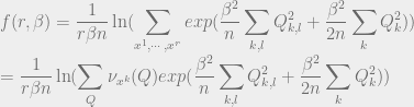
![f(r, \beta) = \frac{1}{r\beta n}\ln{{\mathbb{E}}}_Y[Z^r]](https://s0.wp.com/latex.php?latex=f%28r%2C+%5Cbeta%29+%3D+%5Cfrac%7B1%7D%7Br%5Cbeta+n%7D%5Cln%7B%7B%5Cmathbb%7BE%7D%7D%7D_Y%5BZ%5Er%5D&bg=eeeeee&fg=666666&s=0&c=20201002)
![{{\mathbb{E}}}_Y[Z^r] = \int_Y \sum_{x^1, \cdots, x^r} exp(\beta \sum_k <Y, X^k> \mu(Y) dY\\ = \int_Y \sum_{x^1, \cdots, x^r} exp(\beta <Y, \sum_k X^k>) \mu(Y) dY](https://s0.wp.com/latex.php?latex=%7B%7B%5Cmathbb%7BE%7D%7D%7D_Y%5BZ%5Er%5D+%3D+%5Cint_Y+%5Csum_%7Bx%5E1%2C+%5Ccdots%2C+x%5Er%7D+exp%28%5Cbeta+%5Csum_k+%3CY%2C+X%5Ek%3E+%5Cmu%28Y%29+dY%5C%5C+%3D+%5Cint_Y+%5Csum_%7Bx%5E1%2C+%5Ccdots%2C+x%5Er%7D+exp%28%5Cbeta+%3CY%2C+%5Csum_k+X%5Ek%3E%29+%5Cmu%28Y%29+dY&bg=eeeeee&fg=666666&s=0&c=20201002)
We then simplify the above expression with a technical claim.
Claim 2. Let 

for some constant 

Denote 

To understand the term inside exponent better, we can rewrite the inner
sum in terms of overlap between replicas:
![{{\mathbb{E}}}_Y[Z^r] = \sum_{x^1, \cdots, x^r} exp(\frac{\beta^2}{n}{{\|{X}\|_{F}}}^2 + \frac{\beta^2}{2n} <a^Ta, X>)](https://s0.wp.com/latex.php?latex=%7B%7B%5Cmathbb%7BE%7D%7D%7D_Y%5BZ%5Er%5D+%3D+%5Csum_%7Bx%5E1%2C+%5Ccdots%2C+x%5Er%7D+exp%28%5Cfrac%7B%5Cbeta%5E2%7D%7Bn%7D%7B%7B%5C%7C%7BX%7D%5C%7C_%7BF%7D%7D%7D%5E2+%2B+%5Cfrac%7B%5Cbeta%5E2%7D%7B2n%7D+%3Ca%5ETa%2C+X%3E%29&bg=eeeeee&fg=666666&s=0&c=20201002)

where the last equality follows from rearranging and switch the inner
and outer summations.
Using a similar trick, we can view the other term as

Note that 

overlaps between the
In the end, we get for any integer
Our goal becomes to approximate this quantity. Intuitively, if we think
of 


with 
expect ![Q_{j, k} \in [\pm \frac{1}{n}]](https://s0.wp.com/latex.php?latex=Q_%7Bj%2C+k%7D+%5Cin+%5B%5Cpm+%5Cfrac%7B1%7D%7Bn%7D%5D&bg=eeeeee&fg=666666&s=0&c=20201002)

remaining part, We find the correct
Observe that by introducing a new variable 

using the property of gaussian intergal (Equation 4):

Replace each 
have (Equation 2):

![\begin{gathered} {{\mathbb{E}}}[Z^r] = \sum_{x^1, \cdots, x^r} exp(\frac{\beta^2}{n}\sum_{k, l}Q_{k, l}^2 + \frac{\beta^2}{2n}\sum_k Q_k^2) \label{e:2}\\ = C\sum_{x^1, \cdots, x^r} \exp(\beta^2 n)\int_{Z_{k, l}}exp(-\frac{n}{4}\sum_{k \neq l}Z_{k, l}^2 - \frac{n}{2}\sum_k Z_k^2 + \beta \sum_{k \neq l}Y_{k, l}Q_{k, l} + 2\beta\sum_kZ_k Q_k) dZ \\ =C\exp(\beta^n) \int_{Y_{k, l}}exp(-\frac{n}{4}\sum_{k \neq l}Y_{k, l}^2 - \frac{n}{2}\sum_k Z_k^2 + \ln(\sum_{x_1,\cdots, x_r}exp(\beta \sum_{k\neq l}Y_{k, l}Q_{k, l} + 2\beta\sum_kY_k Q_k)) dY \label{e:2}\end{gathered}](https://s0.wp.com/latex.php?latex=%5Cbegin%7Bgathered%7D+%7B%7B%5Cmathbb%7BE%7D%7D%7D%5BZ%5Er%5D+%3D+%5Csum_%7Bx%5E1%2C+%5Ccdots%2C+x%5Er%7D+exp%28%5Cfrac%7B%5Cbeta%5E2%7D%7Bn%7D%5Csum_%7Bk%2C+l%7DQ_%7Bk%2C+l%7D%5E2+%2B+%5Cfrac%7B%5Cbeta%5E2%7D%7B2n%7D%5Csum_k+Q_k%5E2%29+%5Clabel%7Be%3A2%7D%5C%5C+%3D+C%5Csum_%7Bx%5E1%2C+%5Ccdots%2C+x%5Er%7D+%5Cexp%28%5Cbeta%5E2+n%29%5Cint_%7BZ_%7Bk%2C+l%7D%7Dexp%28-%5Cfrac%7Bn%7D%7B4%7D%5Csum_%7Bk+%5Cneq+l%7DZ_%7Bk%2C+l%7D%5E2+-+%5Cfrac%7Bn%7D%7B2%7D%5Csum_k+Z_k%5E2+%2B+%5Cbeta+%5Csum_%7Bk+%5Cneq+l%7DY_%7Bk%2C+l%7DQ_%7Bk%2C+l%7D+%2B+2%5Cbeta%5Csum_kZ_k+Q_k%29+dZ+%5C%5C+%3DC%5Cexp%28%5Cbeta%5En%29+%5Cint_%7BY_%7Bk%2C+l%7D%7Dexp%28-%5Cfrac%7Bn%7D%7B4%7D%5Csum_%7Bk+%5Cneq+l%7DY_%7Bk%2C+l%7D%5E2+-+%5Cfrac%7Bn%7D%7B2%7D%5Csum_k+Z_k%5E2+%2B+%5Cln%28%5Csum_%7Bx_1%2C%5Ccdots%2C+x_r%7Dexp%28%5Cbeta+%5Csum_%7Bk%5Cneq+l%7DY_%7Bk%2C+l%7DQ_%7Bk%2C+l%7D+%2B+2%5Cbeta%5Csum_kY_k+Q_k%29%29+dY+%5Clabel%7Be%3A2%7D%5Cend%7Bgathered%7D&bg=eeeeee&fg=666666&s=0&c=20201002)
where
To compute the integral in (Equation 2), we need to cheat a little bit and take
is defined as
This is the second assumption made in the replica method and it is
commonly believed that switching the order is okay here. Physically,
this is plausible because we believe intrinsic physical quantities
should not depend on the system size.
![f(\beta) = \lim_{n \to \infty}\lim_{r \to 0}\frac{1}{r\beta n}\ln {{\mathbb{E}}}_Y[Z(\beta, Y)^r]](https://s0.wp.com/latex.php?latex=f%28%5Cbeta%29+%3D+%5Clim_%7Bn+%5Cto+%5Cinfty%7D%5Clim_%7Br+%5Cto+0%7D%5Cfrac%7B1%7D%7Br%5Cbeta+n%7D%5Cln+%7B%7B%5Cmathbb%7BE%7D%7D%7D_Y%5BZ%28%5Cbeta%2C+Y%29%5Er%5D&bg=eeeeee&fg=666666&s=0&c=20201002)
Now the Laplace method tells us when
Theorem 1 (Laplace Method). Let 

where 


Fix a pair of 
what’s left to do is to find the critical point of
derivatives gives
where


We now need to find a saddle point of
do that, we choose to assume the order of the replicas does not matter,
which is refer to as the replica symmetry case. 1 One simplest form
of 


Plug this back in to Equation 2 gives: (Equation 3)
![\label{e:3} {{\mathbb{E}}}[Z^r] = C\exp(\beta n)\exp(-\frac{n}{2}(\frac{r^2 - r}{2})y^2 - \frac{n^2}{2} + \ln(\sum_{x^i}\exp(y\beta\sum_{k \neq l}Q_{k, l} + 2y\beta \sum_k Q_k))](https://s0.wp.com/latex.php?latex=%5Clabel%7Be%3A3%7D+%7B%7B%5Cmathbb%7BE%7D%7D%7D%5BZ%5Er%5D+%3D+C%5Cexp%28%5Cbeta+n%29%5Cexp%28-%5Cfrac%7Bn%7D%7B2%7D%28%5Cfrac%7Br%5E2+-+r%7D%7B2%7D%29y%5E2+-+%5Cfrac%7Bn%5E2%7D%7B2%7D+%2B+%5Cln%28%5Csum_%7Bx%5Ei%7D%5Cexp%28y%5Cbeta%5Csum_%7Bk+%5Cneq+l%7DQ_%7Bk%2C+l%7D+%2B+2y%5Cbeta+%5Csum_k+Q_k%29%29&bg=eeeeee&fg=666666&s=0&c=20201002)
To obtain
(Equation 3) as 
in (Equation 4) we have
![\lim_{r \to 0}\frac{1}{r}\ln(\sum_{x^i}\exp(y\beta\sum_{k \neq l}Q_{k, l} + n\beta \sum_k Q_k)) = -\beta + {{\mathbb{E}}}_{z \sim \mathcal{N}(0, 1)}[\log(2cosh(y\beta + \sqrt{y\beta}z))]](https://s0.wp.com/latex.php?latex=%5Clim_%7Br+%5Cto+0%7D%5Cfrac%7B1%7D%7Br%7D%5Cln%28%5Csum_%7Bx%5Ei%7D%5Cexp%28y%5Cbeta%5Csum_%7Bk+%5Cneq+l%7DQ_%7Bk%2C+l%7D+%2B+n%5Cbeta+%5Csum_k+Q_k%29%29+%3D+-%5Cbeta+%2B+%7B%7B%5Cmathbb%7BE%7D%7D%7D_%7Bz+%5Csim+%5Cmathcal%7BN%7D%280%2C+1%29%7D%5B%5Clog%282cosh%28y%5Cbeta+%2B+%5Csqrt%7By%5Cbeta%7Dz%29%29%5D&bg=eeeeee&fg=666666&s=0&c=20201002)
Using the fact that we want the solution to minimizes free energy,
taking the derivative of the current
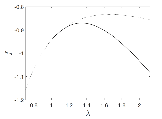
which matches the fixed point of AMP. Plug in
the solid line is the curve of
dotted line is the curve given by setting all variables
![\frac{y}{\beta} = n{{\mathbb{E}}}_z[tanh(y\beta + \sqrt{y\beta}z)]](https://s0.wp.com/latex.php?latex=%5Cfrac%7By%7D%7B%5Cbeta%7D+%3D+n%7B%7B%5Cmathbb%7BE%7D%7D%7D_z%5Btanh%28y%5Cbeta+%2B+%5Csqrt%7By%5Cbeta%7Dz%29%5D&bg=eeeeee&fg=666666&s=0&c=20201002)
References
-
Turns out for this problem, replica symmetry is the only case. We
will not talk about replica symmetry breaking here, which
intuitively means we partition replicas into groups and re-curse. ↩
