Prices, Competition, and Captivity

Imagine that two technology companies A and B sell similar products (e.g. phones) and they compete for customers. Some customers are loyal to one company or the other, perhaps because they already have products from company A that are incompatible with offerings from company B or visa-versa.  Other customers are willing to buy either product and will shop for the lowest price.  Each company must set a price for their product, but they cannot discriminate between the market segment that is loyal to their brand (i.e., captive) and the market segment that is shared with the competition.

The market structure in this scenario pits the two companies against each other in a pricing game.  Each company must select a price and then obtains revenue determined by the buyers’ decisions. What would be an equilibrium of this game? In the absence of captive markets, this is the classic Bertrand competition scenario, and the two companies will undercut each other’s prices all the way down to the marginal cost of production.  What happens when some buyers are captive?

Consider, as an example, the simplest scenario that generalizes Bertrand competition: two sellers A and B share a market of size 1, while additionally seller A has a captive market of size 1. Each buyer is interested in an item and is willing to pay 1 for it, while the sellers can produce any number of items at cost 0. Seller A cannot price discriminate so he must post the same price for buyers in both markets. Buyers at the shared market buy from the seller that offers the lower price. The seller are now in a game in which each needs to post one price and each seller’s utility is her revenue.

Let’s work out the Nash equilibrium in this instance.  Unlike Bertrand competition, it is not an equilibrium for both sellers to choose price 0: seller A could choose instead to sell at price 1, abandoning the market shared with B but extracting high revenue from the captive market.  This further implies that there are no pure strategy equilibria in this game, since if one seller sets a single price then the other would simply undercut it, or jump the price up to 1.  We therefore consider mixed equilibria, where each seller chooses a distribution over prices.  The following properties of a mixed equilibrium are easily derived:

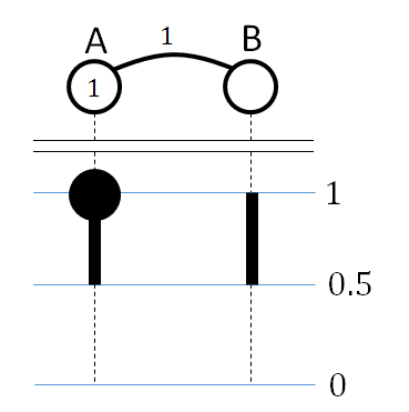
• Regardless of seller B’s choices, seller A is always better off choosing price 1 than any price less than 0.5; the support of her strategy therefore lies in [0.5, 1].
• Since seller B would never choose a price less than A’s minimum price, seller B will select prices from [0.5, 1] as well.
• Neither seller can have an “atom” (i.e., a price selected with positive probability), except perhaps seller A at price 1, since otherwise the other seller would choose to undercut.  Likewise, neither seller can have a “hole” (a range in which she does not bid, lying between her lowest and highest potential bids).
• Seller A must always lose the shared market at the highest price in her support, so this highest bid must be 1 and her equilibrium utility is u_A(1)=1.
• Every price in some seller’s support gives the seller the same utility. Indifference of A between price 1 and the lowest price in her support implies that this lowest price must be 0.5, as with that price she wins both markets. We conclude that the support of both sellers’ strategies is exactly [0.5, 1].

A summary of these facts about the equilibrium is illustrated in Figure 1.  This information – the sellers’ supports, and which sellers can have atoms at price 1 – is an equilibrium “sketch.”

We can now solve for the equilibrium price distributions given the sketch.   It turns out that this step is easy: the equilibrium condition requires that each seller is indifferent over her support, and this requirement uniquely determines the distribution over prices for the sellers.  In our example (writing F_A and F_B for the CDFs for the sellers), if seller B chooses price p then she gets utility u_B(p) = p(1-F_A(p)).  Since we also have u_B(p) = u_B(0.5) = 0.5 (since B is guaranteed to win the shared market at this price), we conclude F_A(p) = 1 – 1/(2p) for p in [0.5, 1].  We can similarly use the indifference of seller A to conclude F_B(p) = 2 – 1/p for p in [0.5, 1].

It may be surprising that seller B obtains positive utility, despite having access only to a shared market.  Contrast this with what would happen if seller B were to gain access to the captive market of A: the sellers would be put in a classic Bertrand competition and the equilibrium prices would go down to 0.  In other words, given the choice, seller B prefers to yield part of her market to seller A.

The simple example above carries much of the intuition for equilibria in more general networks.  Let us present an abstract model that generalizes the scenario above to a setting where there may be many sellers and many buyers, with access to different sets of sellers.  Sellers are represented by nodes in a hyper-graph, and each hyper-edge represents a population of buyers that can only buy from its incident nodes. A hyper-edge has a weight, corresponding to the size of its population. Every buyer is interested in one item, and is willing to pay at most 1 for it. Each seller can produce any number of items, at a cost of zero. Sellers simultaneously post prices; each seller posts a single price that is offered to all buyers in incident edges. Each buyer then buys from the incident seller that offers the cheapest price (as long as it is at most 1). We will focus on the case that the hyper-graph is actually a graph; that is, each buyer has access to at most two sellers. In our joint paper with Noam Nisan we study this Bertrand Network model. In what follows, we highlight some properties of Bertrand networks.

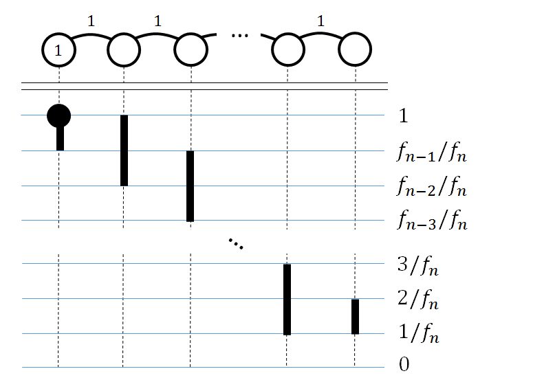
Uniqueness: a line with a single captive market.  Imagine generalizing the two-seller example to a line of n sellers, with each consecutive pair sharing a market and only the first seller having a captive market, all markets of size 1.  It turns out in this case that there is a unique equilibrium, with supports illustrated in Figure 2.  In this equilibrium, the utility of the i-th seller is given by f_{n-i+1}/f_n, where f_i is the i’th Fibonacci number.  (To see this, note that setting price f_{n-i+1}/f_n causes seller i to certainly win one shared market and certainly lose the other).  In particular, the utilities decay exponentially in distance from the captive market.  Moreover, uniqueness is no accident: in any tree network with a single captive market, all equilibria are utility-equivalent.

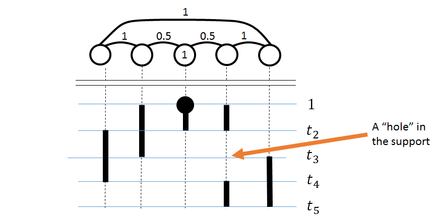
Non-uniqueness and holes: the case of cycles.  One might ask if the equilibrium uniqueness result for tree networks holds more generally, but this is not the case.  In networks with cycles, it may be that there are multiple (non-utility-equivalent) equilibria of the resulting pricing game.  Moreover, these equilibria can exhibit “holes” — that is, the support of an equilibrium strategy may not be a contiguous range of prices.  An example of both these phenomena is given in Figure 3.  In this example the network is symmetric with respect to reflection around the center node, but the equilibrium sketch is not.  There are therefore at least two equilibria, the one illustrated and its reflection, and these equilibria are not utility equivalent from the perspective of the non-center sellers.

Computing equilibria: we leave the problem of the complexity of equilibria computation open.  If we are given a network instance and an equilibrium sketch (i.e., the supports of an equilibrium strategy profile), it is computationally easy to reconstruct the equilibrium strategies.  This is so because we can formulate the indifference conditions as a set of linear constraints, with variables corresponding to probability masses between transition points in the support of some sellers, and then use the indifference to compute the exact CDFs on these intervals.  This suggests an obvious question: how difficult is it to compute an equilibrium sketch?  We leave this as an open problem.  In fact, we also leave open the question of whether, for a given network, there always exists an equilibrium sketch of polynomial size (that is, a sketch that has only polynomially many holes).

Further open questions: All of the above applies only to graphical networks.  What can we say about more general hypergraphs?  We also consider only a very simple model of price competition where marginal costs of production are zero and buyers have infinite demand at the smallest price; classic Bertrand competition extends to more general supply and demand curves, so we could imagine extending this analysis in a similar fashion.

Moshe Babaioff and Brendan Lucier