High frequency moments via max-stability

In this post, I will present what I think is a simple(r) algorithm for estimating the $k>2$ frequency moment, or simply the $\ell_k$ norm of a vector, in the sketching/streaming model. In fact, the algorithm is just a weak embedding of $n$ -dimensional $\ell_k$ into $\ell_\infty$ of dimension $m=O(n^{1-2/k}\log n)$ (this viewpoint spares me from describing the streaming model precisely).

What do I mean by a weak embedding? We will get a randomized linear map $f:R^n\to R^m$ such that, for any $x,x'\in R^n$ , we have that the image $\|f(x)_i-f(x')_i\|_\infty=\max_i |f(x)-f(x')|$ is a constant approximation to $\|x-x'\|_k=(\sum_i |x_i-x'_i|^k)^{1/k}$ with some 90% probability. Since $m\ll n$ , the embedding is actually dimensionality-reducing.

Before I jump into the algorithm, let me mention that the algorithm is essentially based on the approach from a paper joint with Robi Krauthgamer and Krzysztof Onak, and also the paper by Hossein Jowhari, Mert Saglam, and Gabor Tardos. At least our paper was itself inspired by the first (near-)optimal algorithm for frequency moment estimation of Piotr Indyk and David Woodruff (later improved by Lakshminath Bhuvanagiri, Sumit Ganguly, Deepanjan Kesh, and Chandan Saha).

The algorithm. Let $x$ be the input vector of dimension $n$ . The algorithm just multiplies $x$ entry-wise by some scalars, and then folds the vector into a smaller dimension $m$ using standard hashing. Formally, in step one, we compute $y$ as

$y_i= x_i/u_i^{1/k}$

where random variable $u_i$ is drawn from an exponential distribution $e^{-u}$ . In step two, we compute $z$ from $y$ using a random hash function $h:[n]\to [m]$ as follows:

$z_j = \sum_{i:h(i)=j} \sigma_i \cdot y_i$

where $\sigma_i$ are just random $\pm 1$ .

$f(x)=z$ is the output, that’s it. In matrix notation, $f(x)=PDx$ , where $D$ is a diagonal matrix and $P$ is a sparse $0/\pm1$ “projection” matrix describing the hash function $h$ .

Of course the fun part is to show that this works (simple algorithm is not necessarily simple analysis). I’ll give essentially the entire analysis below, which shouldn’t be bad.

Analysis. We’ll first see that the infinity norm of $y$ is correct, namely approximates $\|x\|_k$ , and then that the infinity norm of $z$ is correct as well (both with constant approximation with constant probability of success). In other words, step one is an embedding into $\ell_\infty$ , and step two is dimensionality reduction.

The claim about the infinity norm of $y$ follows from the “stability” property of the exponential distribution: if $u_1,\ldots u_n$ are exponentially distributed, and $\lambda_i>0$ are scalars, then $\min\{u_1/\lambda_1,\ldots u_n/\lambda_n \}$ is distributed as $u/\lambda$ where $u$ is also an exponential and $\lambda=\sum_i \lambda_i$ .

Now, applying this stability property for $\lambda_i=|x_i|^k$ we get that $\|y\|_\infty^k=\max_i |x_i|^k/u_i$ is distributed as $\|x\|_k^k/u$ .

Note that we already obtain a weak embedding of $\ell_k^n$ into $\ell_\infty^n$ (i.e., no dimensionality reduction). We proceed to show that the dimension-reducing projection does not hurt.

We will now analyze the max-norm of $z$ . The main idea is that the biggest entries of $y$ will go into separate buckets, while the rest of the “stuff” (small entries) will give a minor contribution only to each bucket. Hence, the biggest entry of $y$ will stick out in $z$ as well (and nothing bigger will stick out), preserving the max-norm. For simplicity of notation, let $M=\|x\|_k$ , and note that the largest entry of $y$ is about $M$ (as we argued above).

What is big? Let’s say that “big” is an entry of $y$ such that $|y_i|\ge M/\log n$ . With good enough probability, there are only at most $O(\log^k n)\ll \sqrt{m}$ such big items (because of exponential distribution), so they will all go into different buckets.

Now let’s look at the extra “stuff”, the contribution of the small entries. Let $S$ be the set of small entries. Fix some bucket index $j$ . We would like to show that the contribution of entries from $S$ that fall into bucket $j$ is small, namely, less than $\approx M$ (the max entry of $y$ ).

Let’s look at $z'_j=\sum_{i\in S:h(i)=j} \sigma_i y_i$ . A straight-forward calculation shows that the expectation of $z'_j$ is zero, and the variance is $E_{h,\sigma}[{z'}_j^2]=E_h[\sum_{i\in S:h(i)=j} y_i^2]\le \|y\|_2^2/m$ . If only we now could show that $\|y\|_2^2 \ll M^2m$ , we would be done by Chebyshev’s inequality…

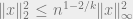How do we relate $\|y\|_2$ to $M=\|x\|_k$ ? Here comes the exponential distribution at rescue again. Note that $E[\|y\|_2^2]=\sum_i x_i^2\cdot E[1/u_i^{2/k}]=\sum_i x_i^2\cdot O(1)=O(\|x\|_2^2)$ since the expectation $E[1/u^{2/k}]$ for an exponentially distributed $u$ is constant. Together with standard inter-norm inequality that $\|x\|_2^2\le n^{1-2/k}\|x\|_\infty^2$ , we have that $E[\|y\|_2^2]\le O(n^{1-2/k} M^2)$ .

Combining, we have that $E[{z'}_j^2] \le O(n^{1-2/k} M^2/m)\le O(M^2/\log n)$ , which is enough to apply Chebyshev’s and conclude that the “extra stuff” in bucket $j$ is $|z'_j|\le o(M)$ with constant probability.

We are almost done except for one issue: we would need the above for all buckets $j$ , and, in particular, we would like to have $|z'_j|\ll M$ for a fixed $j$ with high probability (not just constant). To achieve this, we use a stronger concentration inequality, for example the Bernstein inequality, which allows us exploit the fact that 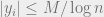$|y_i|\le M/\log n$ for $i\in S$ to achieve a high-probability statement.

Discussion. The use of “stability” of exponential distribution is similar to Piotr Indyk’s use of $p$ -stable distributions for sketching/streaming $\ell_p$ , $p\in(0,2]$ , norms. Note that $p$ -stable distributions do not exist for $p>2$ ; so here the notion of “stability” is slightly different. In the former, one uses the fact that for random variables $v_1,\ldots v_n$ , which are $p$ -stable, we have that $\sum \lambda_i v_i$ is also $p$ -stable with well-controlled variance. In the latter case, we use the property that the max of several “stable” distributions is another one: $\max \lambda_i/u_i$ is distributed as $\lambda/u$ (i.e., $1/u$ is “max-stable”). Note that this is useful for embedding into $\ell_\infty$ . As it turns out, such a transformation does not increase the $\ell_2$ norm of the vector much, allowing us to do the dimensionality reduction in $\ell_\infty$ .

For streaming applications, the important aspects are the small final dimension $m=O(n^{1-2/k} \log n)$ and the linearity of $f$ . This dimension of $m$ is optimal for this algorithm.

UPDATE: a preliminary write-up with formal details is available here.

	Mostafa Touny on Avi wins the Turing, TCS for…
	Harvard Professors o… on Open letter to the Harvard…
	Harvard Professors o… on Open letter to the Harvard…
	Harvard, we have a p… on Letter to the Harvard Corporat…
	Eitan bachmat on Letter to the Harvard Corporat…

High frequency moments via max-stability

Published by Alex Andoni

Leave a comment Cancel reply

Share this:

Related

Published by Alex Andoni

Leave a comment Cancel reply