Higher Lower Bounds: Just Ask for More!

In memory of Mihai Pătraşcu.

Continuing the spirit of the previous post, in this post I will describe a specific technique for proving lower bounds for (static) data structures, when the space is (near) linear. This technique was introduced in the paper by Mihai and Mikkel Thorup, called “HIGHER lower Bounds for Near-Neighbor and  F u r t h e r  Rich Problems”.

Let’s start from the basics: how do we prove any data structure lower bound to start with? First of all, let’s fix the model: the cell-probe model, which is essentially the strongest of all, introduced by Yao in ’81. Here, the memory is composed of cells, each of bits, and the processor obtains the query and subsequently probes different cells of the memory. The cell-probe complexity is the number of cells to be probed to answer the query correctly for some problem .

To be specific, here’s a sample problem , called the partial match. Dataset is a set of points , the query , and the data structure is required to report whether the query matches any of the points in the set, assuming that can match either 0 or 1. We think of dimension as for . For example, there is a simple solution with space, using only one probe, by computing an index table. (The parameter is usually thought of as polynomial in the dimension .)

A very common approach to a lower bound in the cell probe model is via asymmetric communication complexity, as suggested by Peter Bro Miltersen, Noam Nisan, Shmuel Safra, and Avi Wigderson in ’95. The idea is to formulate the problem as a communication game. Alice represents the processor, and thus gets the query. Bob represents the memory, and hence gets the data structure. Their “communication game” is as one would expect: Alice and Bob communicate until they solve the problem. The asymmetry part comes from the fact that the input sizes are unequal, and hence we are attentive to how much information is sent from Alice to Bob, termed , and the other way around, termed (in contrast to the total communication).

[MNSW’95] proved the following. Suppose there exists a solution to the data structure question, with space and probes. Then, there is a solution to the corresponding communication game, with and (obtained by the straight-forward simulation of the data structure). Hence, if we prove a lower bound for the communication game version, we get a data structure lower bound. For instance, for partial match, one can prove that: any protocol must have either or else for any . Putting these together, we conclude that , or, equivalently, that . For any polynomial space, the lower bound is thus . Note that, here, the most important constraint is on — the constraint on is obviously not satisfied for low number of probes.

Such a lower bound is nice but it cannot quite differentiate between, say, cubic space versus linear space: just triple the query time and we’ve reduced the space to linear! This is of course not what happens in real data structures (I wish!). Part of the trouble comes from the fact that the communication game is more powerful than the data structure. In particular, Bob can remember what Alice has previously asked — which is clearly not the case in a data structure.

How can we prove a (higher) lower bound for a linear space data structure? Here come Mihai and Mikkel.

The idea is to ask for more! In particular, they consider several queries at the same time, by taking the -sum of the problem. One intuition goes as follows: partition the data set into a bunch of small problems, namely of them, each of size for some constant , and each of queries goes to its own mini-problem. Then, we prove a space lower bound of for each of these mini-problems, and then show that the total space has to be the sum: . The intuition is good, but how to make this formal? In particular, why does the space of the data structure has to add up?

Here is a different, more formal intuition.  Again take the -sum. Define the “data structure” problem as: given instances, of size , what is the space versus cell-probe complexity trade-off ? The “communication game” variant is the natural one: Alice gets queries, Bob gets data structures, etc. As before, if there is a solution for the data structure setting, then there is a solution for the communication game.

Now comes the most interesting part (of this post at least): there actually exists a communication game that does a more efficient simulation than one which would just multiply all communication by ! Namely, consider one probe (for all queries at the same time). By previous argument, Alice would send bits ( probes into space ). One can do better: sending is sufficient since Alice has just to specify the cells out of which she wants to read. Note that, when and are close to , the log factor is substantially less than before. All in all, Alice and Bob can achieve communication only and .

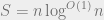
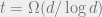
To obtain a Higher lower bound, it only remains to prove a communication complexity lower bound for the -sum communication game. In particular, one hopes to prove a lower bound for the -sum of the problem, which does multiply the required communication by . Essentially, we want a statement of the type: either Alice has to send bits or Bob has to send bits. Putting two such statements together, [PT’06] obtain a data structure lower bound for partial match of . Or, for near-linear space , we have a lower bound of whenever (contrast this with the earlier bound of for any polynomial space).

Final remarks. The original paper used a slightly weaker communication complexity lower bound for the partial match, which yielded a slightly weaker data structure lower bound. It has been strenghened to the above bound by Mihai using the LSD reduction (featured in the previous post), as well as by Rina Panigrahy, Kunal Talwar, and Udi Wieder in 2008, who have introduced a different method for showing lower bounds for near-linear space data structures. I should also mention that Mihai and Mikkel have actually first obtained a separation between polynomial and (near-)linear space in their earlier paper on predecessor search.

Good luck to all who have to deliver on promises made on June 26th.