September 17, 2026 · Boaz Barak · Scribe notes by Daniel Schwartz, Dev Desai, and Ed Gerrard
Lecture Video: https://youtu.be/Lp_e8Ts5-nE
Slides: Presentation slides
Authors’ Intro
Daniel Schwartz: I’m a second-year MS/MBA student. I worked as a PM at multiple early-stage startups, most recently a startup focused on data privacy for AI use with sensitive enterprise data. I’m looking to broaden my AI knowledge as I build my own startup.
Dev Desai: I’m a first year Master’s Student studying Computational Science and Engineering. Broadly, my interests span ML algorithms & diffusion, LLM research (scaling laws, ICL), and mechanistic interpretability. I’m taking this course because I want to gain a broader scope of the safety field than just what I encounter through mech interp.
Ed Gerrard: I am a second year MS/MBA student. I’ve worked as a SWE/PM at Spotify and Soundtrap, focussing on audio experiences for consumers. I’m excited to learn more about safety and alignment within AI and am particularly interested in understanding how these understandings can relate to musicians and their workflows.
Outline
This post covers three parts of the session:
1. Pre-reading: readings on GPU performance, transformer arithmetic and inference, instruction tuning, RLHF, policy gradients, reasoning models, on-policy distillation, and the SmolLM3 training recipe.
2. Boaz’s lecture: why deep learning favors simple methods that scale, how transformers are shaped by GPUs, a single picture of pretraining and post-training, the math behind SFT and policy gradients, and safety training with deliberative alignment.
3. Experiment: study of when natural-language filler text gives a model extra room to compute.
I. Pre-reading
This week had nine readings. The first three are about hardware and the arithmetic of transformers, the next three about post-training, and the last three about reasoning models and full training pipelines.
1. Horace He, “Making Deep Learning Go Brrrr From First Principles”
Deep learning performance depends on three factors: compute, memory bandwidth, and overhead. To speed up a model, we must understand the bottleneck. Improving memory when the constraint is compute will have negligible impact on performance. Trial-and-error solutions will not resolve model performance; a structured approach based on first principles is needed.
2. Austin et al., “All the Transformer Math You Need to Know”
The size, training cost, and memory needs of a transformer can be estimated based on the transformer design. For example, training cost is roughly 6 × parameters × tokens FLOPs, two for the forward pass and four for the backward pass.This chapter gives practical tools for deciding what scale of a model is feasible and which components will become expensive.
3. Austin et al., “All About Transformer Inference”
During inference, latency and throughput put different pressure on a system. The inference process can be split into a compute-bound prefill phase and a memory-bandwidth-bound generation phase. The hardware constraints shift depending on a variety of factors like quantization, batch size, caching, and attention across the two stages of inference.
4. Nathan Lambert, “Instruction Fine-Tuning”
Instruction fine-tuning trains a model to respond to requests beyond just predicting the next word in a sentence. The process involves training on structured question-answer formats; notably, chat templates with designated roles such as system, user, and assistant. Later post-training stages use significantly smaller batch sizes than pre-training runs.
5. Lambert et al., “Illustrating Reinforcement Learning from Human Feedback (RLHF)”
Model performance can improve by training models on human preferences, commonly done by having humans compare different responses and using the comparison as a training signal. RLHF has its challenges: it is costly, human judgements are imperfect and inconsistent, and a learned score is only a proxy for what people want. RLHF has three stages: start from a pre-trained model, train a reward model on human rankings of its output, then fine-tune the model against that reward.
6. OpenAI Spinning Up, “Part 3: Intro to Policy Optimization”
Policy optimization involves training an AI to make decisions through trial and error. The policy takes action in an environment and observes what follows. Based on the outcomes achieved, parameters are updated so the reward is maximized over time. Policy optimization involves three main ideas. Reward good actions: if an action led to a good overall score, make the AI more likely to pick that action in the future. Reward-the-go: an action you take now cannot affect rewards earned in the past. Compare against expectations: take baselines into account to determine if an action is better or worse than usual.
7. Nathan Lambert, “Reasoning and Inference-Time Scaling”
RLVR uses checkable outcomes, such as math answers or code tests, as a reward signal. This reduces reliance on human preference judgments for those tasks. When tasks are verifiable, models can think for longer when generating an answer. Training on many attempts with verifiable feedback has helped models develop behaviors that productively use additional time spent on generating an answer.
8. Kevin Lu and Thinking Machines Lab, “On-Policy Distillation”
On-policy distillation is an efficient post-training method that combines advantages of reinforcement learning and supervised fine-tuning. A student model generates its own attempts, and a stronger teacher evaluates how it proceeds at each step, giving the student guidance on situations it actually encounters, including its own mistakes. The student learns from the feedback given at every token.
9. Hugging Face, “SmolLM3: smol, multilingual, long-context reasoner”
SmolLM3 is an account of how to build a capable small model through a sequence of choices: what data to train on, how to extend context and reasoning ability, and how to refine the final assistant. It provides the model alongside the blueprint used to create it, demonstrating both a complete recipe and the tradeoffs that must be assessed.
II. Boaz’s Lecture
Why AI is different (0:00)
Boaz opened with a 1989 essay by Edsger Dijkstra. In the physical world, Dijkstra wrote, each scale has its own specialist: the town planner, the architect, the solid-state physicist. A programmer works across the across the whole range from a single bit to hundreds of megabytes, a ratio of about 10⁹, and so has to “think in terms of conceptual hierarchies that are much deeper than a single mind ever needed to face before.”
Boaz argued that AI goes further. A large training run takes around 10²⁵ floating-point operations. When a model misbehaves, the answer can lie anywhere from “We should tell the model we care about its feelings” to “We should change how we quantize real numbers into 4 bits”.
Simple, not stupid, and scales (5:55)
Fig 1 puts a resource such as FLOPs (single arithmetic steps) or dollars on the x-axis, and the intelligence gained per unit of it on the y-axis. Classical machine learning methods are clever and do well on a small budget, but they saturate quickly; i.e. additional spending stops generating returns. Deep learning methods are simple and “not completely stupid,” and their gains stay above zero across many orders of magnitude. Boaz compared classical methods to a clever small investor trying to beat the market, and deep learning to an index fund, which grows steadily and predictably. The goal is a reliable way to “translate money into intelligence of the model,” which can then be scaled up.
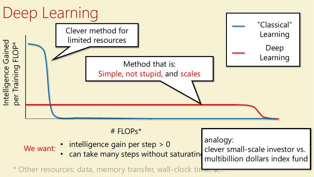
Fig 1. Classical learning versus deep learning, in intelligence gained per FLOP.
Next-token prediction and scaling laws (9:23)
Next-token prediction fits the objective which scales. Improving prediction builds skills and knowledge, any text is training data with a label at every token, and with diverse data the task never saturates. The model turns tokens into vectors, processes them, and turns the final vector into a probability distribution over the next token. Training minimizes the cross-entropy loss, the negative log probability the model gives to the actual next token.
Boaz pushed back on the “stochastic parrot” argument, which says models replay patterns from training data without understanding them. Anything that produces a time series is a next-token predictor, including people, since we speak or act one moment at a time. His rule of thumb is that whenever you hear an argument of the form “LLMs only predict the next word, therefore they can’t do X”, about 90% of the time LLMs can actually do X.
On cost, a transformer takes about 2 FLOPs per parameter per token at inference and about 6 in training, so a fixed compute budget N has to be split between model size and data. Using the same exponent α for both terms, as Boaz did, the Chinchilla scaling law models the loss as aF−α + bD−α + c, where F is the compute per token, which tracks the model size, and D is the number of training tokens. Substitute D = N/F and the loss is lowest where the two terms are equal, at F ≈ √N, so four times the compute buys twice the model and twice the data.
Transformers and GPUs (19:38)
Boaz described two ways to think about designing neural networks. One is to imitate the brain. The other, which he prefers, is to “forget the human brain” and ask what runs well on GPUs. A GPU cluster has many fast cores with limited bandwidth between them. A good architecture should therefore be parallel across tokens, examples, and parameters, do much more computation than communication, and should combine messages by adding them up, so the order doesn’t matter. Matrix multiplication fits well, since multiplying a vector by a d×d matrix takes O(d) communication and O(d²) computation.
A purely linear network meets all of these requirements but can only compute linear functions. Adding a nonlinearity between two matrices gives the feed-forward (MLP) block. Attention comes from giving each position a query for what it wants, a key for what it offers, and a value for what it passes on. How well a query matches a key sets how much one position listens to another.
At inference time, the prompt is processed in parallel (the prefill), and each new token reuses the keys and values already computed for earlier tokens, the KV cache. The same saving is why API providers charge less for input they have already cached.
Next-token prediction has a weakness that Boaz illustrated with two mathematicians. Jean Bourgain’s papers jump between equations, and predicting the next step can take far more thought than a model can do in one token; Terry Tao has described struggling with one of those papers for many months. Tim Gowers is the reverse, he explains hard material so clearly that predicting each step takes little work; the model learns less from it. Tokens vary widely in difficulty, but a transformer spends the same amount of compute on every one.
Pretraining and post-training (31:21)
“Generally you don’t train LLMs,” Boaz said. “You pre-train LLMs and you post-train LLMs.” Pretraining learns the distribution of tokens. Post-training teaches the model to play the role of an assistant.
Boaz framed all of training in one picture (Fig 2). Each token gets a reinforcement. A positive one makes the token more likely given what came before, a negative one makes it less likely, and zero leaves it out of the loss. Tokens are either written by someone else (off-policy) or sampled from the model being trained (on-policy). Pretraining reinforces whole documents. Supervised fine-tuning (SFT) reinforces a pre-written response to a prompt. RL samples the model’s own response and reinforces every token in it with one reward for the whole response. On-policy distillation also samples the model’s response, but has a teacher score each token separately.
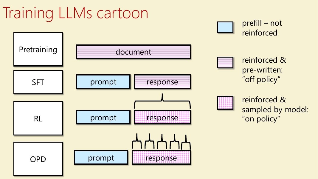
Fig 2. Which tokens each training stage reinforces, and whether they are pre-written or sampled from the model.
On-policy data matters because an off-policy teacher can be a poor match for the model. A weaker teacher can teach worse behavior; a much stronger one may be copied without being understood. A teacher that is merely different from the model can cause regressions or confusion.
From RLHF to verifiable rewards (36:02)
The simplest version of RLHF has a person rate every response during training, which stops working once you remember that “humans need to sleep and pee.” Instead, labs collect human ratings ahead of time and train a reward model to predict them; that model then rates every response. They also ask people to compare two responses rather than score one, since comparing is easier. RLAIF uses an AI to produce the labels, which scales much better but doesn’t tell you exactly what people want.
Reasoning models address the fixed compute per token by thinking before they answer. They are trained with RL from verifiable rewards, where the reward is 1 if the final answer is correct and 0 if not. The reward never looks at the chain of thought, so the thinking is optimized only for reaching good answers.
The math (39:18)
In the second half of the lecture, Boaz went into the mathematical foundations behind these methods, starting from derivatives and gradient descent. The main takeaway from this is the humble chain rule, which allows for the backbone of AI: backpropagation and gradient descent.
Gradient descent updates model parameters in the direction that reduces the loss. Stochastic gradient descent approximates this gradient using a subset of the training data. Backpropagation then uses the chain rule to compute gradients through the many layers of a neural network.
The discussion connected these ideas to SFT (supervised fine tuning). SFT maximizes the log probability assigned to the target responses, which is also equivalent to minimizing the KL divergence between the data and model output distributions. KL divergence is a metric used to measure the distance between two probability distributions. So, SFT encourages the model to reproduce the distribution of the responses in our training data.

Then, we were introduced to two problems that motivate RL: the Bourgain problem, and the Gowers problem. Their implications in AI is that we want to make the model have variable thinking, so we should reward the answer and not the tokens themselves, and have the model learn its own reasoning chain.
RL offers a solution by allowing the model to generate their own reasoning traces and then rewards correct final answers. Our objective function wants to maximize the reward across all prompts and rollouts for each prompt:

Explicitly written,

Then, we take the gradient so we can perform gradient ascent to optimize.

Technically, this formula is correct but not as useful. We want to avoid summing over all y, and want to instead sample and estimate the gradient. To work around this, we employ the log derivative trick:


This is a useful formulation, as we can rewrite it as an expectation. This is the policy gradient.

This leads to an algorithm called REINFORCE, which simply is just sampling a few answers y1,y2…yn, and averaging the inside of the policy gradient as an estimate. After, you can step the weights uphill.

Another note is that we can reduce variance by replacing the reward term with the difference of the average reward of the samples in the step and the reward of the individual rollout.
While SFT trains on predefined examples, REINFORCE trains on responses generated by the model itself, rewarding good responses and discouraging bad ones. Methods like GRPO make this training more stable by comparing and normalizing rewards across multiple responses to the same prompt.
DeepSeekMath suggested that RL primarily makes existing capabilities more reliable, while DeepSeek-R1-Zero provided evidence that RL might also develop more substantial reasoning capabilities.
Distributed Training
We briefly learned about how large models are distributed across GPUs to overcome memory and computational limitations. This is also known as sharding, and it splits many different components of LLMs across devices. You can split individual weight matrices and computations (tensor sharding), different transformer layers (layer sharding), sequence positions (context sharding, useful for long contexts), and experts in mixture-of-expert architectures (expert sharding).
These techniques enable models that would otherwise exceed memory capacity of individual GPUs to be trained and served efficiently.
Safety training (1:08:30)
The final section of the lecture focused on how models are trained to follow safety specifications. Previously safety was focused on user misuse of the model, but safety also shifted towards agents doing harmful things on their own. In general, the goal of AI safety is for the model to follow its safety specification even under worst-case inputs.
Boaz focused on what is called “deliberative alignment,” which teaches reasoning models to explicitly consider safety specifications before responding. This process has two stages: in SFT and in RL (RLHF/RLAIF).
In SFT, a model is given a prompt and safety spec, and then generates a reasoning trace explaining how the spec applies before producing its response. These reasoning traces become training examples so that the model can learn to apply the spec without it being explicitly provided at inference time (Fig 3).
During RL, a reward model that can see the spec checks whether the answer complies. The aim is to teach the model “to not just do the right thing, but do it for the right reason.” Again, this helps efficiency as it pushes the model to produce answers in line with the safety spec without having to always see the spec in context.
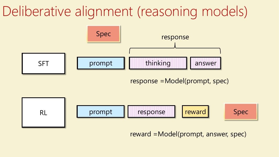
Fig 3. Deliberative alignment. The spec is used to generate the SFT data and to compute the RL reward, but the model being trained never sees it in context.
Next, Boaz went over some brief results. In an example, the model decodes a request and finds that the user wants an untraceable payment method to visit explicit websites. The model reasoned that this request wasn’t necessarily prohibited, but the user’s intent was to hide from the cops which raised concerns, so the model refused.
When applying these safety training processes to o1, the model improved on jailbreak resistance and on avoiding over-refusal at the same time. A version trained only on English data, with no encoded examples, handled encoded and multilingual prompts about as well as one trained on the full dataset, showing that it had become more deeply aligned.
III. Experiment: When Do Natural-Language Fillers Become Computational Substrate?
Experiment group: Andrea Chen, Andrew Wu
Background
The group built on [Brauer et al. (2026)], which found that adding filler, such as a long string of periods, after a question can improve a model’s accuracy even with chain of thought turned off. This suggests the model can use filler positions to do computation it would otherwise write out. That work and related studies used a multishot format, where the model sees example problems, each with the same filler and a correct answer, before the test problem.
Setup
The group asked whether filler with meaning works the same way, and whether its position matters. They compared three kinds of filler: counting, true statements, and false statements, all matched for token length. Each was placed before the question, in the middle of it, or after it. They tested DeepSeek V4 Flash and DeepSeek V3 (0324) on 300 systems-of-equations problems in the 10-shot format.
Results
Filler after the question improved accuracy on both models for all three kinds of filler. With counting filler placed after the question, accuracy rose from 52% to 69.3% on V4 Flash and from 33.3% to 56% on V3-0324. Filler before the question lowered accuracy. Filler in the middle did not help either, even though the model could in principle have started on the part of the problem it had already seen.
To see whether the model was computing in the filler positions, the group decoded the model’s intermediate states with the logit lens, J-lens, and R-lens. Because the filler repeated across examples, the lenses mostly predicted the next filler word, so the group subtracted the average representation across problems to isolate the problem-specific signal. This turned up intermediate values from the solution, such as 74, 148, and 172. With activation patching, they replaced the filler activations of one problem with those of another problem that used the same filler. When the later layers were patched, the model gave the other problem’s answer; when only the earlier layers were patched, it did not.
Follow-up
One concern with the 10-shot setup is that after seeing the same statements ten times, the model might simply learn to ignore them. To investigate this, the group ran a 3-shot experiment comparing repeated statements with new statements in each example.
They found that repeated true and false statements both improved accuracy, while new false statements reduced it. New true statements had little effect on V4 Flash but reduced accuracy on V3.
This suggests that repeated text can become space for computation, regardless of whether it’s true or false. In contrast, unfamiliar false statements may distract the model because it still processes them as factual claims. However, this doesn’t explain why new true statements also hurt V3. The group emphasized that these findings were preliminary, based on only two models and a few days of experimentation.


